Understanding LoRA
I finally got time to have some deep dives. Happy Christmas!
RAM Usage During Training
Training large-scale machine learning models e.g. LLMs, requires significant compute resources. Here’s a breakdown of the possible memory usage (RAM) at various stages of the classic training process, based on the pseudocode below:
1 | model = Model() |
Key Components of Memory Usage
Model Parameters: These are the trainable weights of the model, which need to be stored in memory throughout the training process. The size is proportional to the number of parameters in the model.
Model Gradients: Gradients for each parameter are computed during backpropagation and stored temporarily for the optimizer to update the weights.
Optimizer States: Optimizers like Adam maintain additional states, including:
First-order momentum: Tracks the moving average of gradients.
Second-order momentum: Tracks the moving average of squared gradients.
Both momentum terms have the same size as the model gradients.
Activations: Activation outputs from the forward pass are stored for use during backpropagation, where the Hessian matrix is multiplied with the activations. The memory required for activations can be substantial, especially as batch size increases. While the size of parameters, gradients, and optimizer states remains constant, activation memory scales directly with batch size.
Other Overheads: Temporary buffers and memory fragmentation during computation also contribute to RAM usage.
Memory Calculation Examples
Gradients and Parameters:
For 70B model, using 32-bit floating-point precision (FP32): \[ 70\times10^9\times4 \text{ bytes}\times2 =521.5\text{GM} \] This accounts for the weights and their corresponding gradients.
Optimizer State:
Adam optimizer requires two additional states (first and second-order momentum), each the same size as the gradients: \[ 70\times10^9\times4 \text{ byte}\times2 =521.5\text{GM} \]
Activations:
For 70B model with a hidden size of 8192, 80 layers, and FP32 precision, each token’s activation memory: \[ 8192\times80\times4\times12 \text{ bytes/token}=30\text{ MB/token} \]
Simple Strategies for Reducing Memory Usage
- Activation Checkpointing: Instead of storing all activation outputs, recompute activations during backpropagation as needed. This significantly reduces activation memory at the cost of additional compute time.
- Mixed Precision Training (FP16): Use 16-bit floating-point precision (FP16) instead of FP32 for model weights, gradients, and activations. This halves the memory requirements without substantial accuracy loss when done correctly.
LoRA
Adapters
The original adapter was introduced in 2019 in the paper "Parameter-Efficient Transfer Learning for NLP". It's a small, additional module added to a pre-trained model to adapt it to a new task without significantly changing the original model parameters.
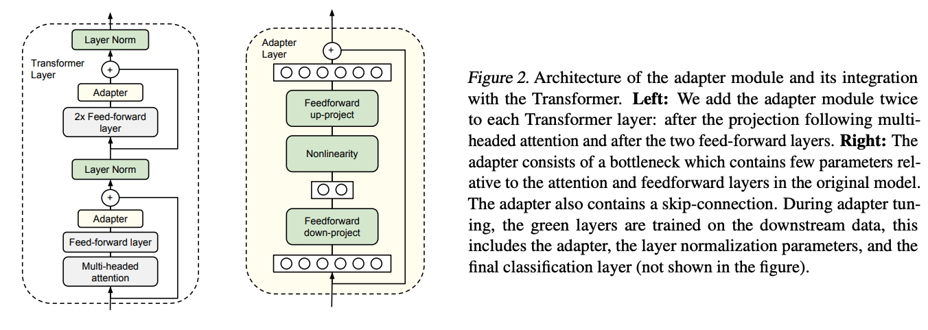
Adapters generally reduce training latency compared to full fine-tuning because only a small number of parameters (those within the adapter modules) are updated during training. This reduction in trainable parameters leads to lower computational overhead and faster convergence in many cases. Additionally, adapters allow for larger batch sizes due to reduced memory usage, which can further accelerate training
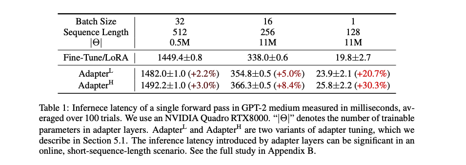
However, adapter layers increase inference latency because they are added sequentially and cannot be parallelized. This issue becomes more pronounced with small batch sizes or when using sharded models, such as GPT-2. Techniques like layer pruning or multi-task settings can mitigate but not completely eliminate this latency.
As shown in the experiment results below, inference latent can be significant (Source: LoRA paper):
LoRA Basics
LoRA (Low-Rank Adaptation) was introduced by a Microsoft team in 2021 in the paper LoRA: Low-Rank Adaptation of Large Language Models. The main idea of LoRA is to enable efficient fine-tuning of large pre-trained models by introducing low-rank trainable matrices into the model’s architecture, while keeping the original model weights frozen. This approach significantly reduces the number of trainable parameters and computational requirements compared to full fine-tuning, without compromising performance.
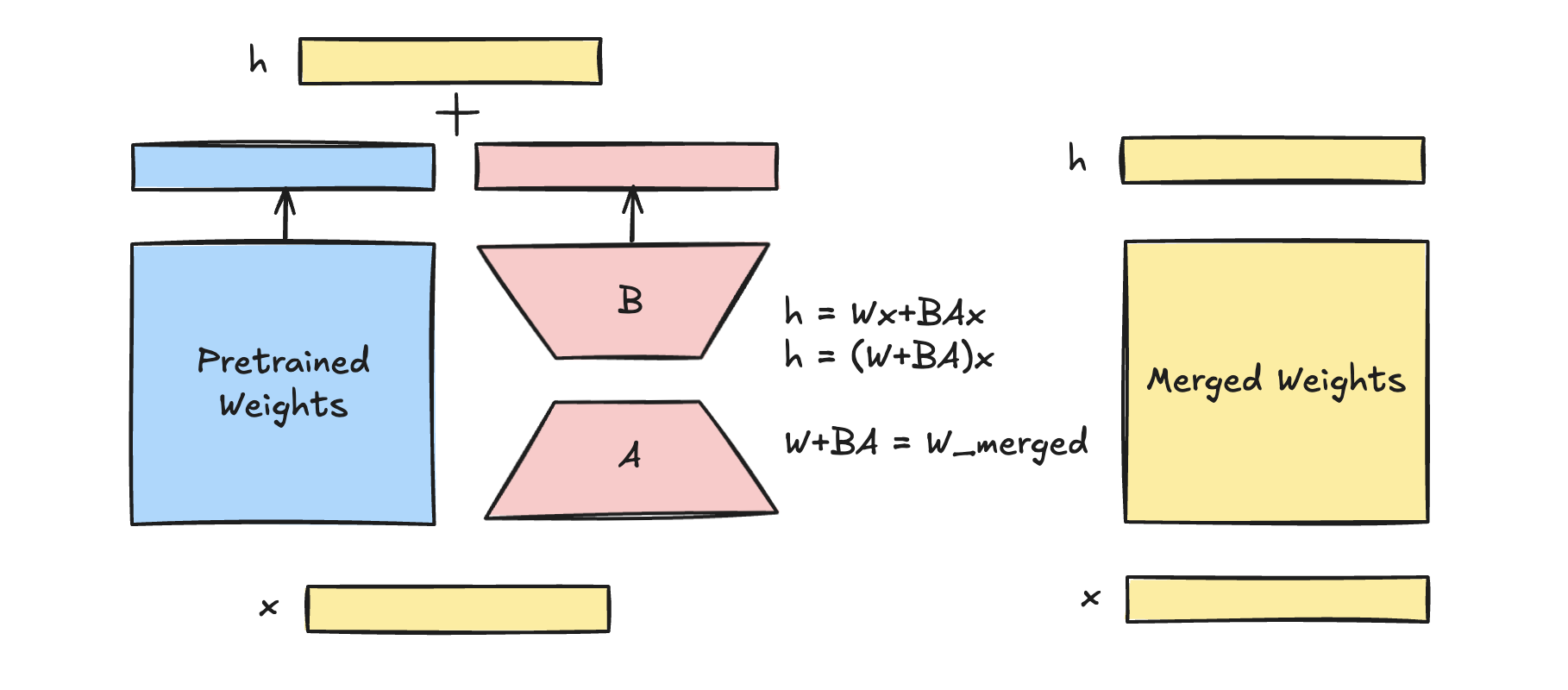
LoRA approximates weight updates in neural networks using low-rank matrix factorization. Instead of updating the full weight matrix \(W\) , it introduces two smaller trainable matrices \(A\) and \(B\) with size \((r \times d)\) and \((d \times r)\). These matrices have much fewer parameters, as their rank \(r\) is much smaller than the dimensions of \(W\). Instead of training \(\Delta W\), LoRA trains the parameters in \(A\) and \(B\). This can be written in formula: \[ h=W_0x + \Delta Wx = W_0x + BAx \] where \(W_0\) is original prerained weight matrix in size \((d\times d)\) which is frozen during training; \(\Delta W\) is in \((d \times d)\) as well computed by \(BA\). \(x\) is a new input with size \((1 \times d)\).
At the start of the training process, the matrix $ A $ is randomly initialized following a normal distribution \(\mathcal{N}(0, \sigma^2)\), while the matrix $ B $ is initialized as a zero matrix. In the initial round, this setup results in $ BA = 0 $, leading to $ h = W_0x $. This initialization strategy ensures stability by preventing significant deviations of $ W_0 $ from its original state.
LoRA is a groundbreaking method with a lot of benefits:
- Parameter Efficiency: By training only the low-rank matrices, LoRA reduces the number of updated parameters resulting in lower memory usage and faster training.
- Frozen Pre-trained Weights: The original pre-trained weights remain unchanged, preserving the model’s general-purpose knowledge and avoiding catastrophic forgetting.
- No Inference Latency Overhead: Unlike adapters, LoRA does not add additional layers to the model. The low-rank matrices can be merged back into the original weight matrix after fine-tuning, ensuring no additional inference latency.
- Versatility: LoRA can be applied to various architectures (e.g. transformers) and tasks, making it a flexible solution for adapting large models like GPT-3 or RoBERTa to specific use cases.
LoRA Usage
The Microsoft developers of LoRA created a Python package called loralib to
facilitate the use of LoRA. With this library, any linear layer
implemented as nn.Linear() can be replaced by
lora.Linear(). This is possible because LoRA is designed to
work with any layer involving matrix multiplication. The
lora.Linear() module introduces a pair of low-rank
adaptation matrices, which are used to modify the original weight matrix
by applying a low-rank decomposition.
1 | # ===== Before ===== |
Before training the model, all non-lora matrix should be fixed and only LoRA matrices should be set as trainable. Training loops can run as usual.
1 | import loralib as lora |
When saving model checkpoints during LoRA fine-tuning, only the LoRA-specific parameters need to be saved, not the entire large pre-trained model. This results in significantly smaller checkpoint files and more efficient storage.
1 | # ===== Before ===== |
Implementation of LoRA - lora.Linear()
Let's take a deep dive into the lora.Linear() source
code:
The lora.Linear class builds upon
torch.nn.Linear(). It retains the original weight matrix $
W $ as initialized in
nn.Linear.__init__(self, in_features, out_features), and
introduces two additional LoRA matrices: self.lora_A and
self.lora_B. The matrix self.lora_A has
dimensions of $ (r, ) $, while self.lora_B has dimensions
of $ (, r) $. These matrices are used to adapt the original weight
matrix through low-rank decomposition.
1 | class Linear(nn.Linear, LoRALayer): |
In the forward() function, it implements \(h=W_0x + \Delta Wx = W_0x+ BAx\).
There is a flag variable called self.merge which is use
to flag whether it's doing inference or training. Recall that the
original weight matrix remaining unchanged during LoRA training is a key
feature of the LoRA - pre-trained weights are freezed and instead small,
low-rank matrices are trained to approximate updates.
- During inference, if
merge_weightsis set toTrue, the low-rank updatesself.lora_B @ self.lora_Aare added directly to the frozen pre-trained weights (self.weight). This avoids the need for separate computations of LoRA updates during forward passes, improving efficiency. - During training, if
merge_weightsis enabled and weights were previously merged, the updates are subtracted fromself.weightto revert it to its original frozen state. This ensures that gradients are not incorrectly computed on the merged weights.
1 | class Linear(nn.Linear, LoRALayer): |