Understanding QLoRA

Posted on 2024-12-26

QLoRA is never as simple as a single line of code. Let's start from the scaling law...

Neural Scaling Law

In the context of LLMs, a scaling law refers to an empirical relationship that describes how the performance of a model changes as key resources—such as model size (number of parameters), dataset size, and computational power—are scaled up or down. These laws provide insights into how increasing these factors impacts model accuracy, efficiency, and generalization capabilities.

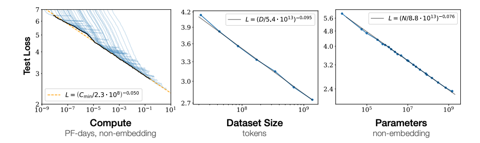
Compute, dataset size, and model size are not independent of each other. Data size and model size together determine compute. The paper "Algorithmic progress in language models" came up with a rule \(C=6ND\) where \(C\) is compute, \(N\) is model size, and \(D\) is data size.

According to the paper "Scaling Laws for Neural Language Models" and "Training Compute-Optimal Large Language Models", below are the key takeaways of scaling laws for LLMs:

Performance Improvement: Model performance often improves predictably with increases in size, data, and compute, typically following a power-law relationship.
Diminishing Returns: Beyond certain thresholds, the benefits of scaling diminish, meaning further increases in resources yield smaller performance gains.
Trade-offs: Effective scaling requires balancing resources like model parameters and training data. For example, the "Chinchilla scaling law" highlights that increasing data size can sometimes yield better results than merely increasing model size in compute-constrained settings.

These observations are critical for LLM research:

Guidance for Optimization: Scaling laws help researchers allocate resources efficiently and predict the outcomes of scaling efforts, guiding both model design and training strategies. For example, within fixed computational constraints and limited training duration, scaling laws provide a principled approach to determining the optimal model size that minimizes test loss.
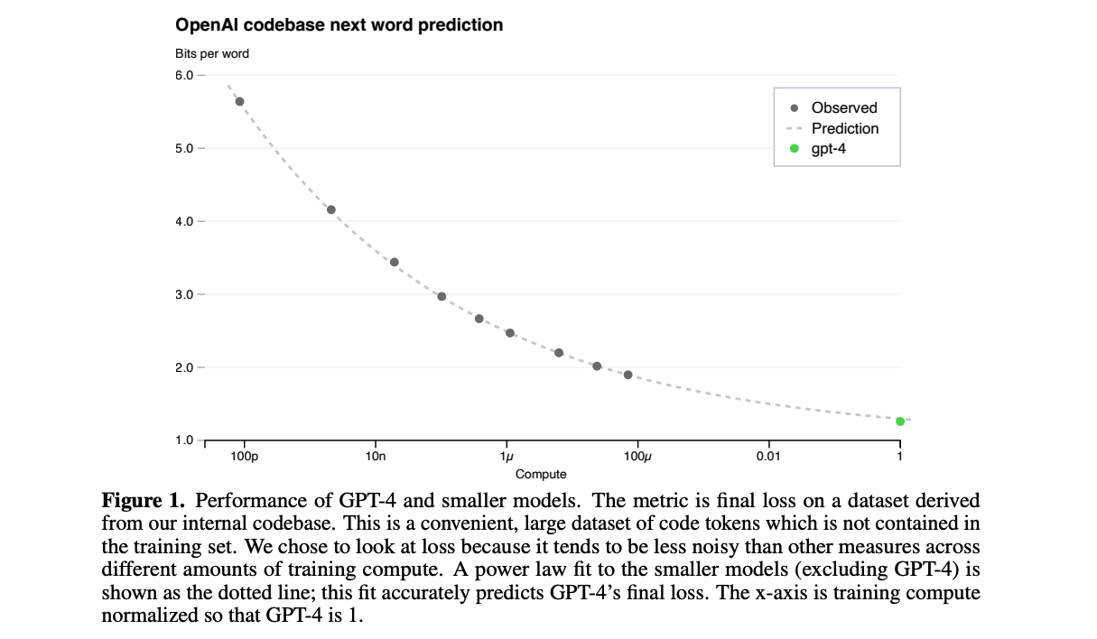
Predicting model performance: As demonstrated in GPT-4 Technical Report, by fitting the scaling law to the loss of smaller models, the loss of a bigger model can be predicted accurately.

The scaling law overlooks a critical practical consideration, which can lead to misconceptions. While it suggests that larger models yield better performance, in reality, the primary compute bottleneck lies in inference rather than training. Training compute is often less constrained because training time can be extended, but deployment costs are significantly higher. From a practical standpoint, a more efficient approach is to train a smaller model for an extended period, as this substantially reduces inference compute requirements.

Quantization

Background

As the scaling law suggested, when training a LLM, reducing the number of parameters is probably not an optimal idea for saving computational resource. Luckily, neural nets are robust in low precision, which means lowering precision won't reduce much model performance.

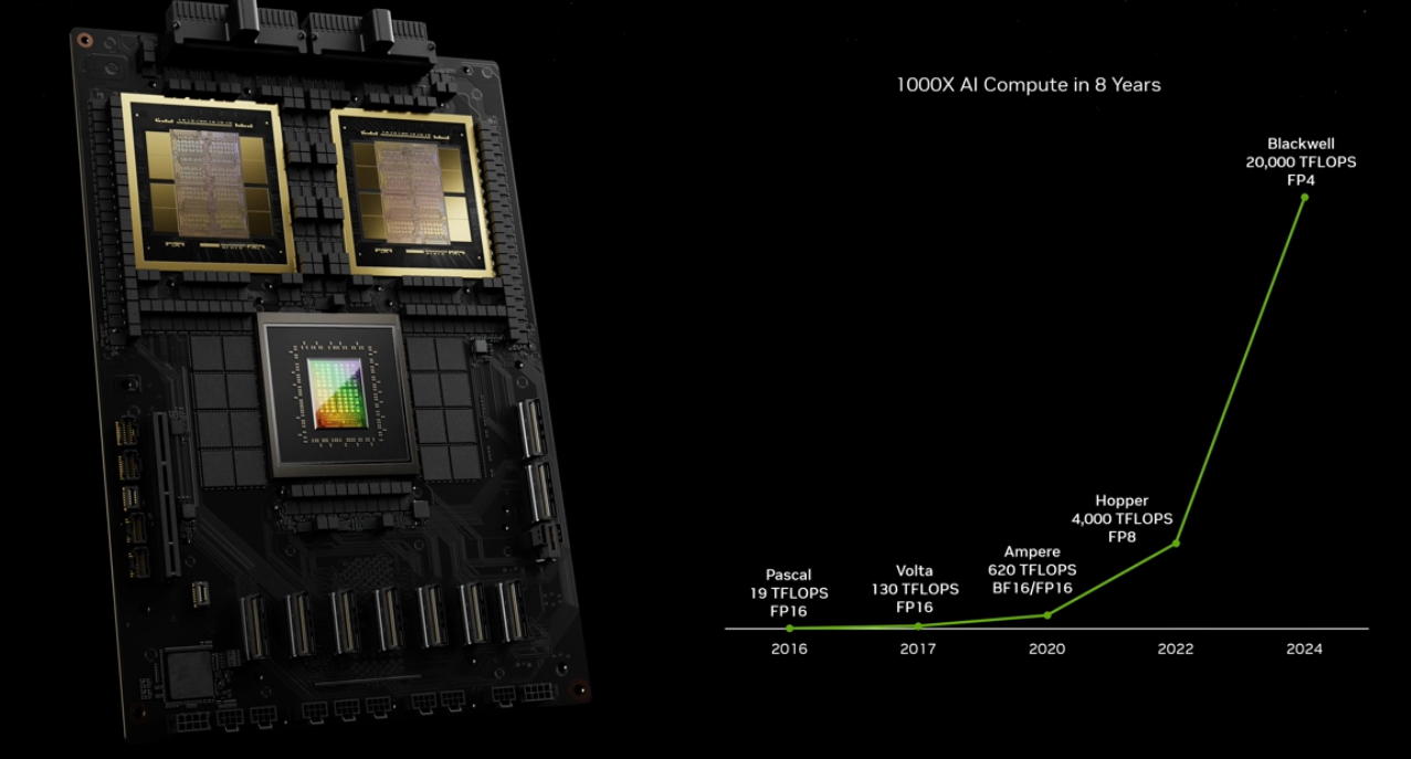
In GTC March 2024 Keynote with NVIDIA CEO Jensen Huang, Jensen stated that NVIDIA has achieved 1000X increase compute power for the past 8 years, faster than Moore’s law. It can be noticed that in the graph they show TFLOPs on FP8 precision in 2022 and TFLOPs on FP4 precision in 2024. This is a trick because it's easier to achieve higher TFLOPs when the precision is lower. And it shows that there is a trend in hardware industry to achieve higher TFLOPs in low precision.

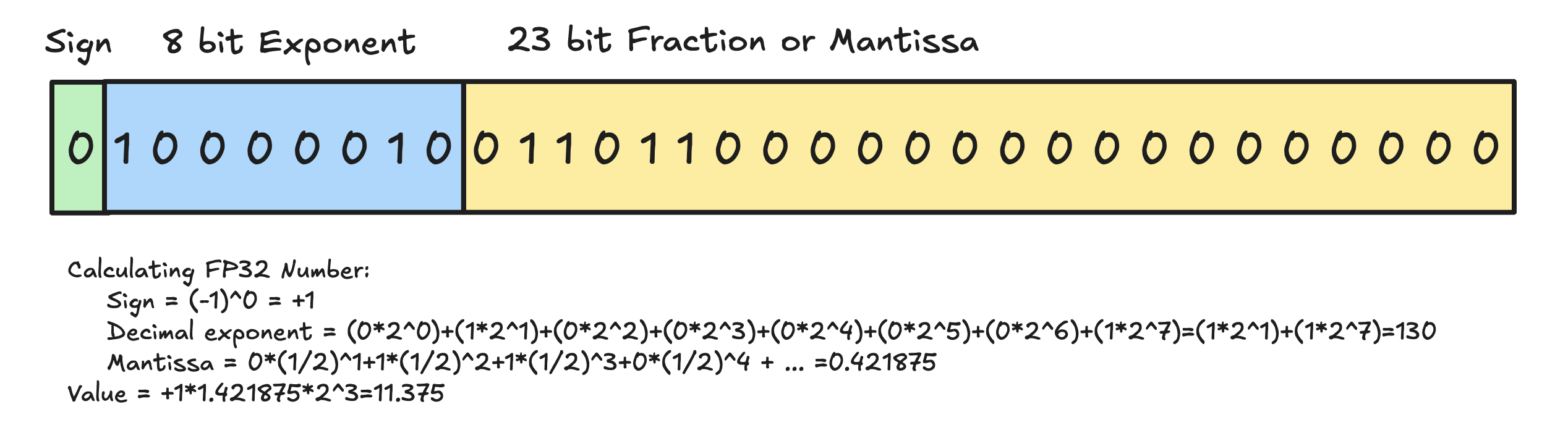
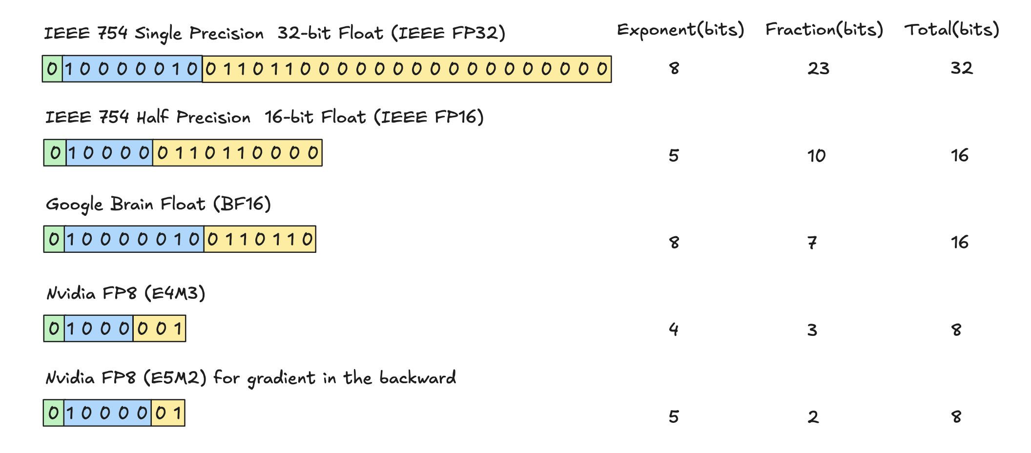
Data Structure - FP32

The IEEE 754 single-precision floating-point format (FP32) represents a 32-bit number in binary form. It is used for approximating real numbers. The FP32 format has three components:

Sign bit (1 bit): Indicates whether the number is positive (0) or negative (1).
Exponent (8 bits): Encodes the exponent, biased by 127 to allow both positive and negative exponents.
Mantissa or Fraction (23 bits): Represents the significant digits of the number.

The formula for FP32 is as follows: \[ \text{Value} = (-1)^{\text{Sign}} \times (1.\text{Mantissa}) \times 2^{\text{Exponent}-127} \] Following this formula, we can calculate FP32 number. Below is an example:

FP32 provides a wider range and higher precision, making it suitable for tasks requiring numerical accuracy, such as training large-scale deep learning models. FP16, with its lower precision, is optimized for speed and memory efficiency. It is particularly effective for inference tasks or mixed-precision training when paired with FP32 for critical calculations.

However, the overflow problem of FP16 arises due to its limited range of representable values. FP16 has a maximum representable value of 65,504 (\(2^{15} \times (2 - \epsilon)\)), which is much smaller compared to FP32's maximum value of approximately \(3.4 \times 10^{38}\). When computations produce results exceeding this range, an overflow occurs, and the value is replaced by infinity (\(\pm \infty\)). Overflow in FP16 can occur during operations like matrix multiplications or summations in deep learning if the intermediate values exceed the maximum representable range. For example, scaling large tensors or performing high-magnitude computations without normalization can easily result in overflow when using FP16. Overflow leads to loss of numerical accuracy and can destabilize training processes in machine learning. It also affects applications like image processing or scientific simulations where precision and stability are critical.

There are some strategies to mitigate this overflow problem:

Use mixed-precision training. FP16 is used for most computations but critical operations (e.g., gradient accumulation) are performed in FP32 to prevent overflow.
Normalize inputs and intermediate values to keep them within the representable range of FP16.
Use alternative formats like BF16, which have a larger dynamic range while maintaining reduced precision.

Googel Brain BF16 uses the same number of exponent bits as FP32 (8 bits), giving it a much larger dynamic range compared to FP16. This means BF16 can represent very large and very small numbers similar to FP32, avoiding underflows and overflows that are common in FP16. Converting from FP32 to BF16 is straightforward because both formats share the same exponent size. The conversion simply involves truncating the mantissa from 23 bits to 7 bits. BF16 uses only 16 bits per value, reducing memory usage by half compared to FP32. This allows for larger batch sizes and models to fit into limited GPU or TPU memory without sacrificing as much numerical range as FP16 does.

Recently, people have started discussing NVIDIA’s FP8 formats (E4M3 and E5M2) as alternatives to BF16 because of their potential to significantly reduce computational and memory costs while maintaining competitive performance in large-scale machine learning tasks. E4M3 offers higher precision, making it suitable for inference and forward-pass computations where precision is critical. E5M2 provides a wider dynamic range, making it ideal for backward-pass computations during training where large gradients can occur. This flexibility allows FP8 to adapt to different stages of training more effectively than BF16.

NVIDIA’s H100 GPUs are specifically designed to support FP8 with optimized Tensor Cores, achieving up to 9x faster training and 30x faster inference compared to previous-generation GPUs using FP16 or BF16. The Hopper architecture dynamically manages precision transitions (e.g., between FP8 and higher-precision formats like FP32), ensuring stability without manual intervention. "Balancing Speed and Stability: The Trade-offs of FP8 vs. BF16 Training in LLMs" shows that FP8 can deliver similar convergence behavior and accuracy as BF16 in many LLM tasks, with minimal degradation in performance. For inference, FP8 quantization (e.g., E4M3 for KV cache) has been shown to minimally impact accuracy while significantly improving memory efficiency.

However, FP8 comes with challenges such as occasional instability during training (e.g., loss spikes) and sensitivity in certain tasks like code generation or mathematical reasoning. As a result, training LLMs with FP8 precision remains an active area of research and exploration.

Feature	IEEE 754 FP32	IEEE 754 FP16	Google BF16	NVIDIA FP8 E4M3	NVIDIA FP8 E5M2
Bit Width	32 bits	16 bits	16 bits	8 bits	8 bits
Sign Bit	1 bit	1 bit	1 bit	1 bit	1 bit
Exponent Bits	8 bits (bias = 127)	5 bits (bias = 15)	8 bits (bias = 127)	4 bits (bias = 7)	5 bits (bias = 15)
Mantissa Bits	23 bits	10 bits	7 bits	3 bits	2 bits
Dynamic Range	\[ \pm(2^{-126} \text{ to } 2^{127}) \]	\[ \pm(2^{-14} \text{ to } 2^{15}) \]	\[ \pm(2^{-126} \text{ to } 2^{127}) \]	\[ \pm(2^{-6} \text{ to } 2^{7}) \]	\[ \pm(2^{-14} \text{ to } 2^{15}) \]
Precision	~7 decimal digits	~3.3 decimal digits	~2.3 decimal digits	Lower precision	Lower precision
Memory Usage	High	Medium	Medium	Low	Low
Performance	Slower	Faster than FP32	Faster than FP32	Much faster than FP16/BF16	Much faster than FP16/BF16
Applications	Training requiring high precision	Inference or mixed-precision training	Mixed-precision training and inference	Optimized for inference	Optimized for training and inference

Current LLM Training Method in FP8

A training approach has been developed to leverage FP8's efficiency for specific operations while maintaining numerical stability and precision with BF16 for critical components of the model.

During the training process, FP8 is utilized exclusively for computations within the MLP layers, while BF16 is employed for other components of the Transformer architecture, such as Attention, Activation, and Layer Normalization. Both weights and gradients are maintained in BF16 precision.

In the forward pass, weights in BF16 are converted to FP8 (E4M3) for matrix multiplications within the MLP layers. Once the computation is completed, the results are immediately converted back to BF16.
In the backward pass, gradients in BF16 are temporarily converted to FP8 (E5M2) when passing through the MLP layers. After the computations are performed, the results are promptly converted back to BF16.

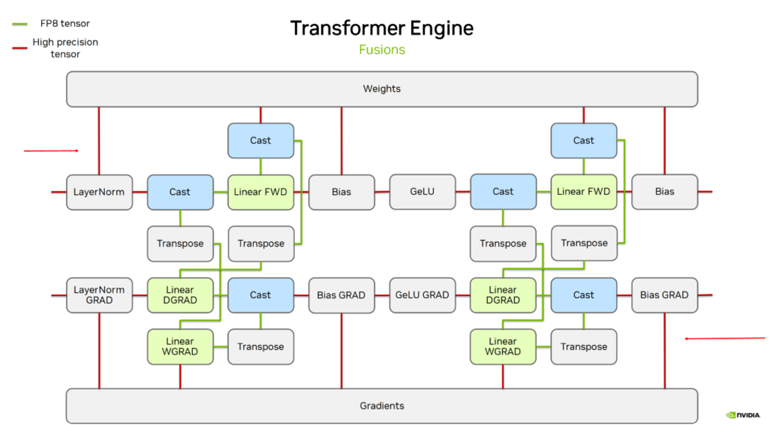
Even when FP8 is used, RAM savings may not be as significant during training because high precision gradients and weights must be maintained in memory to ensure model stability and convergence. The primary benefit of FP8 lies in its ability to reduce memory usage during inference, where weights can be stored in FP8 format, significantly decreasing the memory footprint compared to higher precision formats like FP16 or BF16. Despite this, FP8 is still utilized during training because it allows for faster computations due to its lower precision. This results in accelerated training processes and improved efficiency, especially on hardware optimized for FP8 operations, such as NVIDIA’s H100 GPUs.

Quantization Process

The process of quantization in LLMs refers to a model compression technique that maps high-precision values (e.g., FP32) to lower-precision representations (e.g., INT8 or FP8).

Here is an example of a simple step-by-step quantization from FP16 to INT4:

Range Calculation: Determine the range of FP16 values for the weights or activations. This is typically defined by the minimum and maximum values (\([min, max]\)) in the data.
Scale Factor and Zero-Point Computation: Compute a scaling factor (S) that maps the FP16 range to the INT4 range (\([-8, 7]\) for signed INT4 or \([0, 15]\) for unsigned INT4). Optionally, calculate a zero-point (Z) to handle asymmetric quantization, where zero in FP16 does not align with zero in INT4.

The formula for quantization is: \[ x_q = \text{round}\left(\frac{x}{S} + Z\right) \] where \(x_q\) is the quantized INT4 value, \(x\) is the original FP16 value, \(S\) is the scaling factor, and \(Z\) is the zero-point.
Quantization: Map each FP16 value to its corresponding INT4 representation using the computed scale factor and zero-point. This step reduces precision but compresses the data significantly.

There are different types of quantization:

Asymmetric Quantization vs Summetric Quantization
Uniform Quantization vs Non-uniform Quantization

Quant in General Matrix Multiply (GEMM)

Quantized matrices are stored in memory in their compressed form. During matrix multiplication, these matrices are dequantized back to higher precision (e.g., FP16 or FP32) to perform computations. This process balances memory efficiency with computational precision.

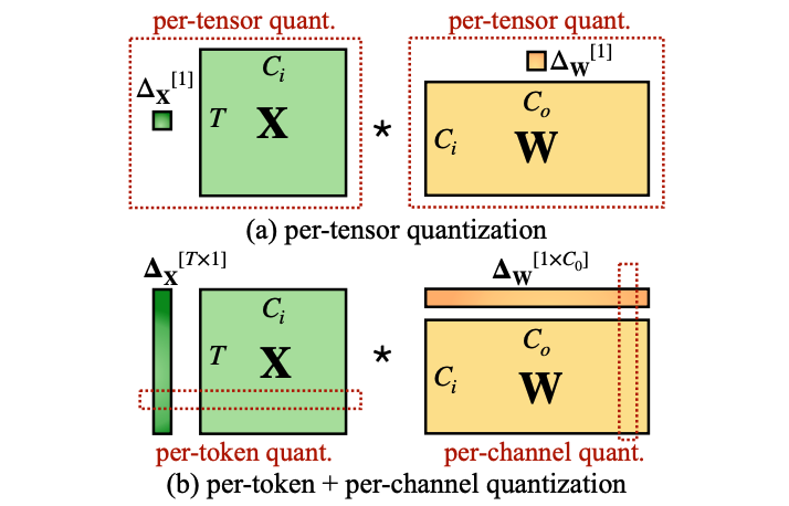
Quantization can be applied at different levels of granularity, which determines how scaling factors are assigned and used. The "SmoothQuant: Accurate and Efficient Post-Training Quantization for Large Language Models" paper introduced several quantization granularity techniques, including per-tensor quantization, per-token quantization, and per-channel quantization:

Per-Tensor Quantization: A single scaling factor is applied to the entire tensor (e.g., a weight matrix or activation matrix). It is highly memory-efficient since only one scaling factor needs to be stored. But it is not recommended in practice because outlier values can dominate the scaling factor, leading to significant quantization errors for the rest of the tensor.
Per-Channel Quantization: Each channel (e.g., each column of a weight matrix or each feature map in activations) has its own scaling factor. Commonly used for weight matrices in neural networks. It mitigates the impact of outliers by isolating them within individual channels, improving quantization accuracy compared to per-tensor methods. But it can introduce computational overhead during dequantization due to the need for multiple scaling factors.
Per-Token Quantization: Each token's activations are assigned a unique scaling factor. Typically used for activations in transformer models. It captures token-specific variations in activations, leading to better precision for tasks with dynamic token distributions. Per-token quantization can be computationally expensive and slower because it requires more scaling factors and additional computations.
Group-Wise Quantization (GWQ): this method groups multiple channels or tokens together and applies a shared scaling factor across the group. It reduces computational overhead compared to per-channel or per-token quantization while maintaining finer granularity than per-tensor methods. It's often used for both weights and activations to strike a balance between accuracy and efficiency.

QLoRA

Fine-Tuning Cost

Comparing cost of full fine tuning, LoRA fine tuning, and QLoRA fine tuning:

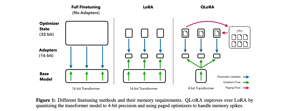
	Full Finetuning	LoRA	QLoRA
Weight	16 bits	16 bits	4 bits
Weight Gradient	16 bits	~0.4 bits	~0.4 bits
Optimizer stage	64 bits	~0.8 bits	~0.8 bits
Adapter weights	/	~0.4 bits	~0.4 bits
Totel	96 bits per parameter	17.6 bits per parameter	5.2 bits per parameter

QLoRA's Contributions

Paper: QLoRA: Efficient Finetuning of Quantized LLMs

4-bit NormalFloat Quantitzation

4-bit NormalFloat Quantitzation adopts the idea of Quantile Quantization which is an information-theoretic method that maps values based on quantiles of the weight distribution. It's a method of data compression where data is quantized (reduced to a smaller set of discrete values) in a way that aims to minimize the information entropy of the resulting data, essentially achieving the most efficient representation possible while still introducing some loss in information, making it a "lossy minimum entropy encoding" technique.

To compute the quantile function for 4-bit NormalFloat (NF4) quantization, the process involves mapping cumulative probabilities to quantization levels optimized for normally distributed data. The quantile function is the inverse of the cumulative distribution function (CDF). For example, as shown in the description, if the probability of \(x < 1.2\) is 0.9, then 1.2 is the corresponding quantile for a cumulative probability of 0.9.

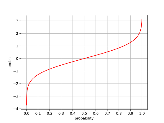
With this quantile function, the probability range from 0 to 1 is divided into 16 equal-sized buckets, as 4 bits can represent \(2^4 = 16\) distinct values. The steps are as follows:

Divide the Probability Range: The range of cumulative probabilities \([0, 1]\) is divided into 16 equal intervals or "buckets." These intervals represent equal portions of the probability mass.
Apply the Quantile Function: For each bucket's cumulative probability value (e.g., \(p_i = \frac{i}{16}\), where \(i \in [1, 15]\)), the corresponding quantile value is computed using the inverse CDF of a standard normal distribution (\(\Phi^{-1}(p_i)\)).
Normalize Quantiles: The resulting quantiles are normalized to fit within a predefined range, typically \([-1, 1]\). This ensures that all quantization levels are symmetrically distributed around zero and fall within a compact range suitable for efficient representation.
Assign NF4 Values: The normalized quantiles become the 16 discrete values used by NF4 to represent weights or activations in a compressed format. These values are spaced closer together near zero (where most of the normal distribution's probability mass lies) and farther apart at the extremes, optimizing precision where it matters most.

Double Quantization

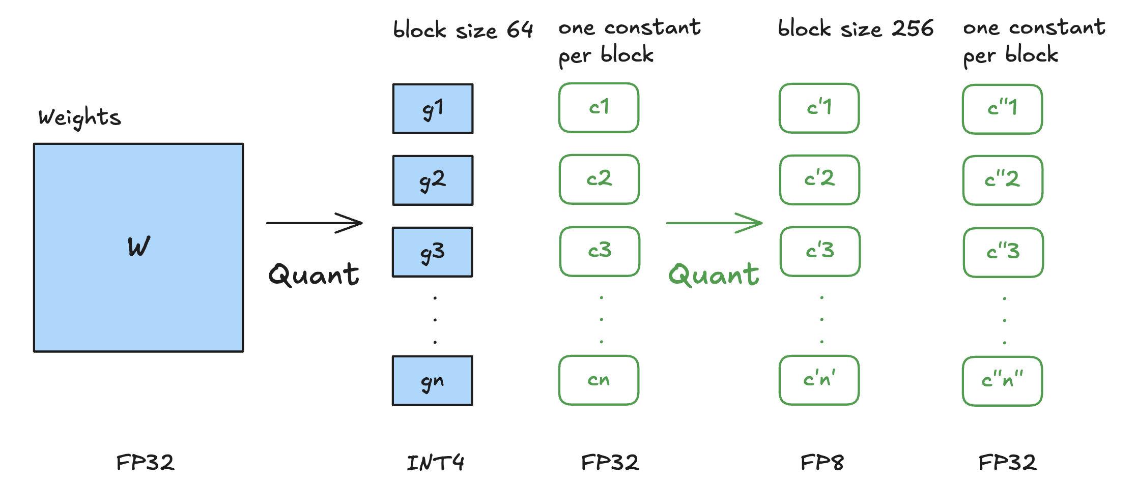
Double Quantization (DQ) as introduced in paper "QLoRA: Efficient Finetuning of Quantized LLMs" is a memory optimization technique that quantizes the quantization constants themselves to further reduce the memory footprint of LLMs. It involves two quantization steps:

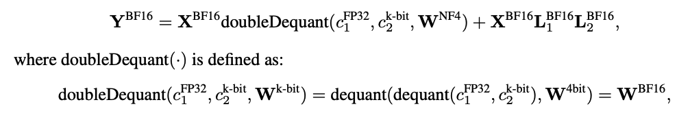
The first quantization involves quantizing the original weights of the model into 4-bit NormalFloat (NF4) format. Weights are divided into small blocks (e.g., 64 elements per block), and each block is scaled by a quantization constant (also known as a scaling factor). This constant ensures that the range of values in each block fits within the representable range of NF4. The quantized weights and their corresponding quantization constants are stored. However, these constants (usually in FP32) can add significant memory overhead.

To calculate the memory overhead: for a block size of 64, storing a 32 bit quantization constant for each block adds \(32/64=0.5\) bits per parameter on average.
The second quantization aims to reduce the memory overhead caused by storing quantization constants. Those quantization constants \(c^{FP32}_2\) are further quantized into 8-bit floating-point values (FP8) with a larger block size (e.g., 256 elements per block). This is a summetric quantization where the mean of the first level factors \(c^{FP32}_2\) is subtracted to center their distribution around zero. This reduces their memory footprint while maintaining sufficient precision for scaling operations. Additionally, another set of quantization constants \(c^{FP32}_1\) is introduced to scale these second-level quantized values.

To calculate the memory savings: after double quantization, the memory footprint per parameter for scaling factors is reduced from \(32/64=0.5\) bits to \(8/64 + 32/(64\times 256)=0.127\) bits per parameter. This results in saving \(0.5-0.127=0.373\) bits per parameter.

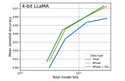
The authors of paper "QLoRA: Efficient Finetuning of Quantized LLMs" compared LLaMA models with different 4-bit data types. They show that the NormalFloat data type significantly improves the bit-for-bit accuracy gains compared to regular 4-bit Floats. While Double Quantization only leads to minor gains, it allows for a more fine-grained control over the memory footprint to fit models of certain size (33B/65B) into certain GPUs (24/48GB). This empirical results show that using FP8 for second-level quantization does not degrade model performance, making it an effective trade-off between precision and memory efficiency.

Paged Optimizers

As described in the QLoRA paper, paged optimizers are a memory management innovation that leverages NVIDIA Unified Memory to handle the memory spikes that occur during gradient checkpointing or when processing large mini-batches with long sequence lengths. NVIDIA Unified Memory allows seamless memory sharing between the GPU and CPU. When the GPU runs out of memory during training, optimizer states (e.g., gradients, momentum, or scaling factors) are paged out (evicted) to CPU RAM. These states are paged back into GPU memory only when needed for computations like gradient updates.

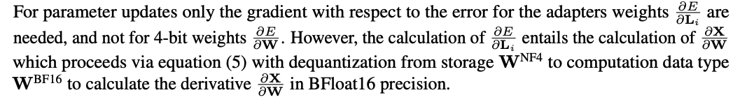
Forward and Backward Implementation

Forward:

Backward:

QLora Usage

QLoRA utilizes bitsandbytes for quantization and is seamlessly integrated with Hugging Face's PEFT and transformers libraries, making it user-friendly. To explore the implementation further, let's dive into the QLoRA code and examine the train() function in qlora.py.

def train():
    hfparser = transformers.HfArgumentParser((
        ModelArguments, DataArguments, TrainingArguments, GenerationArguments
    ))
    model_args, data_args, training_args, generation_args, extra_args = \
        hfparser.parse_args_into_dataclasses(return_remaining_strings=True)
    training_args.generation_config = transformers.GenerationConfig(**vars(generation_args))
    args = argparse.Namespace(
        **vars(model_args), **vars(data_args), **vars(training_args)
    )
    print(args)
    
    checkpoint_dir, completed_training = get_last_checkpoint(args.output_dir)
    if completed_training:
        print('Detected that training was already completed!')

    model, tokenizer = get_accelerate_model(args, checkpoint_dir)

    ......

The get_accelerate_model() function initializes your model and is a crucial component of implementing QLoRA. Notably, within the AutoModelForCausalLM.from_pretrained() method, it loads the quantization configuration through BitsAndBytesConfig. This setup ensures that the model weights are automatically quantized.

def get_accelerate_model(args, checkpoint_dir):

    if torch.cuda.is_available():
        n_gpus = torch.cuda.device_count()
    if is_ipex_available() and torch.xpu.is_available():
        n_gpus = torch.xpu.device_count()
        
    max_memory = f'{args.max_memory_MB}MB'
    max_memory = {i: max_memory for i in range(n_gpus)}
    device_map = "auto"

    # if we are in a distributed setting, we need to set the device map and max memory per device
    if os.environ.get('LOCAL_RANK') is not None:
        local_rank = int(os.environ.get('LOCAL_RANK', '0'))
        device_map = {'': local_rank}
        max_memory = {'': max_memory[local_rank]}


    if args.full_finetune: assert args.bits in [16, 32]

    print(f'loading base model {args.model_name_or_path}...')
    compute_dtype = (torch.float16 if args.fp16 else (torch.bfloat16 if args.bf16 else torch.float32))
    model = AutoModelForCausalLM.from_pretrained(
        args.model_name_or_path,
        cache_dir=args.cache_dir,
        load_in_4bit=args.bits == 4,
        load_in_8bit=args.bits == 8,
        device_map=device_map,
        max_memory=max_memory,
        quantization_config=BitsAndBytesConfig(
            load_in_4bit=args.bits == 4,
            load_in_8bit=args.bits == 8,
            llm_int8_threshold=6.0,
            llm_int8_has_fp16_weight=False,
            bnb_4bit_compute_dtype=compute_dtype,
            bnb_4bit_use_double_quant=args.double_quant,
            bnb_4bit_quant_type=args.quant_type,
        ),
        torch_dtype=(torch.float32 if args.fp16 else (torch.bfloat16 if args.bf16 else torch.float32)),
        trust_remote_code=args.trust_remote_code,
        use_auth_token=args.use_auth_token
    )
    ......

Other than some necessary components like tokenizer, train() gives an option of LoRA in addition to full finetune. It requires setup of LoRA config and get_peft_model function from peft package.

def train():
    ......
  if not args.full_finetune:
          model = prepare_model_for_kbit_training(model, use_gradient_checkpointing=args.gradient_checkpointing)

      if not args.full_finetune:
          if checkpoint_dir is not None:
              print("Loading adapters from checkpoint.")
              model = PeftModel.from_pretrained(model, join(checkpoint_dir, 'adapter_model'), is_trainable=True)
          else:
              print(f'adding LoRA modules...')
              modules = find_all_linear_names(args, model)
              config = LoraConfig(
                  r=args.lora_r,
                  lora_alpha=args.lora_alpha,
                  target_modules=modules,
                  lora_dropout=args.lora_dropout,
                  bias="none",
                  task_type="CAUSAL_LM",
              )
              model = get_peft_model(model, config)
    ......

Not every layers are quantized. QLoRA only quantizes linear projection layers. Some layers like Layer Norm is sensitive to precision, so high precision is required.