Understanding RLHF

Happy New Year (/≧▽≦)/

There is a lot to talk about Reinforcement Learning from Human Feedback (RLHF). How about starting with Reinforcement Learning (RL) basics.

Warning: Extremely long article ahead :)

Overview

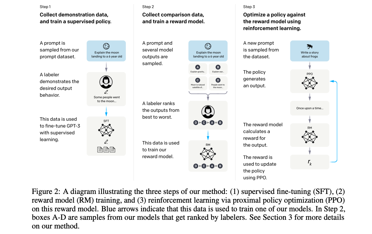
The process of training a model using reinforcement learning from human feedback (RLHF) involves three key steps, as outlined in the paper titled “Training language models to follow instructions with human feedback” by OpenAI.

instructGPT_overview_RLHF

Reinforcement Learning

Introduction

Reinforcement Learning (RL) is a machine learning approach where an agent learns to make decisions by interacting with an environment to maximize cumulative rewards.

The agent is the decision-maker or learner in the RL framework. It performs actions in the environment and learns from the feedback it receives. The environment represents everything external to the agent that it interacts with. It provides feedback in response to the agent’s actions. The state is a representation of the current situation of the environment as perceived by the agent. An action is a decision or move taken by the agent at each step based on its policy (a mapping from states to actions). The reward is a scalar feedback signal provided by the environment to indicate how good or bad an action was in achieving the agent’s goal.

An RL problem is typically formalized as a Markov Decision Process (MDP), which includes:

• States (\(S\)): The set of all possible situations in which the agent can find itself.
• Actions (\(A\)): The set of all possible moves or decisions available to the agent.
• Transition Dynamics (\(P(s'|s,a)\)): The probability of transitioning to a new state \(s'\) given the current state \(s\) and action \(a\).
• Rewards (\(R(s,a)\)): The immediate feedback received after taking action \(a\) in state \(s\).
• Policy (\(\pi(a|s)\)): A strategy that defines how the agent selects actions based on states.

The goal of RL is to find an optimal policy \(\pi^*\) that maximizes cumulative rewards (also called return). This involves balancing short-term rewards with long-term planning using trial-and-error interactions with the environment.

agent_env_rewards_RL_intro

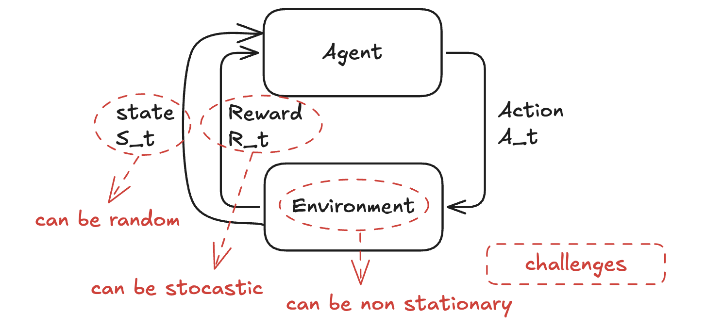
The challenges arised from the nature of environment and its dynamics are non-stationary environments, stochastic rewards, and random states:

• In non-stationary environments, the dynamics of the environment (e.g., transition probabilities or reward functions) change over time. This forces RL agents to continuously adapt their policies, which can lead to a drop in performance during the readjustment phase and forgetting previously learned policies.
• Stochastic rewards occur when the reward function is probabilistic rather than deterministic. This introduces noise into the feedback signal, making it harder for the agent to discern which actions truly lead to higher rewards.
• Random states refer to situations where the agent’s observations are noisy or partially observable, making it harder to infer the true state of the environment. Such randomness complicates policy learning because the agent may need to rely on memory or belief states (e.g., Partially Observable Markov Decision Processes, POMDPs) to make decisions. It increases the dimensionality and complexity of the state space.

The challenges related to algorithmic design and computational feasibility are:

• RL algorithms require a significant amount of interaction with the environment to learn effectively, making them data-intensive. Many RL algorithms, particularly model-free methods like policy gradient techniques, require a large number of samples to converge.
• RL agents face the exploration-exploitation dilemma, where they need to balance trying new actions to discover potentially better rewards (Exploration) and using known actions that yield high rewards (Exploitation).
• Many RL problems involve enormous state and action spaces, such as games like Go or real-world robotics tasks. The exponential growth of possible states and actions makes it computationally challenging for RL algorithms to find optimal solutions.
• Poorly designed rewards can lead to unintended behaviors (e.g., an agent exploiting loopholes in the reward structure). Sparse or delayed rewards make it difficult for the agent to associate its actions with outcomes.
• RL agents often struggle to generalize learned behaviors across different tasks or environments. Agents trained in specific simulations (e.g., driving simulators) may fail to perform well in real-world scenarios due to differences in dynamics, noise, or variability.
• RL algorithms are highly sensitive to hyperparameter choices (e.g., learning rate, discount factor). Poor tuning can lead to slow convergence or failure to converge at all, making training unpredictable and requiring significant expertise.
• RL agents often use complex models (e.g., deep neural networks), making their decisions difficult to interpret. This lack of transparency is problematic in safety-critical applications like healthcare or autonomous driving, where understanding the reasoning behind decisions is essential.

Multi-Armed Bandit (MAB)

The multi-armed bandit (MAB) problem is a classic RL problem that exemplifies the exploration-exploitation tradeoff. It provides a simplified framework for decision-making under uncertainty.

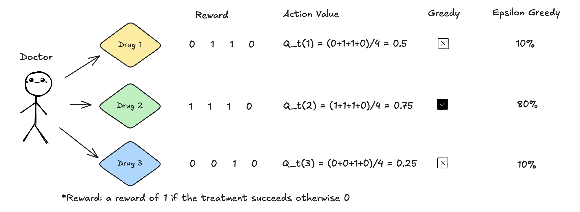
Here is a simple scenario to help understand the Multi-Armed Bandit (MAB) problem. Imagine a doctor has three types of prescription drugs to treat a particular disease and \(N\) patients to treat. At the beginning, the doctor has no knowledge about which drug is the most effective. The goal is to identify the best action—the drug that can cure the highest number of patients.

To achieve this goal, we can define action values as:

\[ Q_t(a) = E[R_t \mid A_t = a], \]

where: - \(R_t\) is a random variable representing whether a patient is cured (reward), - \(a\) is an action, which in this case corresponds to selecting a specific type of drug for the patients.

The best action is the one that maximizes the expected reward:

\[ a^* = \arg\max_a Q(a). \]

It’s important to note that an expectation, \(E[x]\), is typically calculated as:

\[ E[x] = \sum x p(x), \]

where \(p(x)\) represents the probability distribution of \(x\). However, in real-world scenarios where \(p(x)\) is unknown and data is limited, the expectation can be approximated using sample averages:

\[ E[x] \approx \frac{\sum x}{N}, \]

where \(N\) is the total number of observations of \(x\). This approximation process is known as Monte Carlo estimation.

The action value \(Q_t(a)\) can be estimated by Sample-Average Method using the following formula:

\[ Q_t(a) = \frac{\text{Total rewards received when action } a \text{ was taken before time } t}{\text{Number of times action } a \text{ was taken before time } t}. \]

Mathematically, this can be expressed as:

\[ Q_t(a) = \frac{\sum_{i=1}^{t-1} R_i \cdot I_{A_i = a}}{\sum_{i=1}^{t-1} I_{A_i = a}}, \]

where: - \(R_i\) is the reward received at time step \(i\), - \(I_{A_i = a}\) is an indicator function that equals 1 if action \(a\) was selected at time step \(i\) and 0 otherwise.

The best action can be select by Greedy Approach: \[ a^* = \arg\max_a Q(a). \] In our case as demonstrated in the diagram below, after 4 times, \(Q_t(1)=0.5, Q_t(2)=0.75, Q_t(3)=0.25\), the best action is determined by \(\arg \max_a Q_t(a)\) which is Action \(A_2\) (\(a=2\)).

However, this approach has some drawbacks such as small sample size and non-stationary environment (e.g. patients are in different consitions). An intuitive alternative is to give Action \(A_1\) and Action \(A_3\) more opportunities. This is called Exploration - Exploitation Tradeoff, which means to balance trying new actions to discover potentially better rewards (Exploration) and using known actions that yield high rewards (Exploitation).

A better approach is called Epsilon-Greedy Strategy which is a simple yet effective method for addressing the exploration-exploitation tradeoff in RL. It involves:

1. Exploration: With a probability of \(\epsilon\), the agent chooses a random action, allowing it to explore the environment and gather new information.
2. Exploitation: With a probability of \(1-\epsilon\), the agent selects the action that has the highest estimated reward (greedy action) based on its current knowledge.

In our case, let \(\epsilon = 20\%\), \(Q_t(1)\) and \(Q_t(3)\) each is given \(10\%\), and \(Q_t(2)\) is given \(80\%\). The next round (5th) of action is decided by random sampling \(A_1,A_2,A_3\) with probability of \(10\%, 80\%,10\%\). If the sampled action is \(A_1\) and the reward is \(1\), then its action value is updated to be is \(Q_t'(1) = (0+1+1+0+1)/5 =0.6\).

doctor_treatment_example

The pseudo code of Epsilon Greedy Approach is as follows.

# Initialize
for a = 1 to K:
    Q(a) <- 0          # Estimated value of each arm
    N(a) <- 0          # Number of times each arm has been pulled

# Epsilon-Greedy Algorithm
for t = 1 to num_turns:
    with probability ε:
        A <- randomly select an arm (exploration)
    otherwise:
        A <- select the arm with the highest Q(a) (exploitation)

    # Pull the selected arm and observe reward R
    R <- Reward(A)

    # Update the estimates for the selected arm
    N(A) <- N(A) + 1
    Q(A) <- Q(A) + (1 / N(A)) * (R - Q(A))  # Incremental update formula

Note that there is a math trick in the incremental updates Q(A) <- Q(A) + (1 / N(A)) * (R - Q(A)). \[ \begin{equation} \begin{aligned} Q_{n+1} &= {1\over n}\sum^n_{i=1}R_i \space \text{ : average reward in the n+1 iteration}\\ &= {1\over n}(R_n + \sum^{n-1}_{i=1}R_i)\\ &= {1\over n}(R_n + (n-1){1\over n-1}\sum^{n-1}_{i=1}R_i)\\ &= {1\over n} (R_n + (n-1)Q_n)\\ &= {1\over n}(R_n+ n \times Q_n - Q_n)\\ &= Q_n + {1\over n} (R_n - Q_n) \end{aligned} \end{equation} \] The higher the \(\epsilon\), the more opportunities given to actions, and the higher average reward.

epsilon_greedy_method

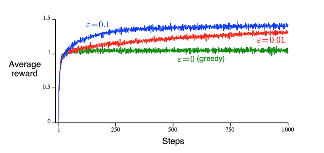
(Source: Reinforcement Learning by Sutton and Barto, Chapter 2)

Agent

Long Term Goal

The goal of Agent is long-term reward \[ G_t = R_{t+1}+R_{t+2}+R_{t+3}+... \] So the objective is expected reward \(E[G_t]\) \[ E[G_t] = E[R_{t+1}+R_{t+2}+R_{t+3}+...] \] There are different types of agent tasks:

• Episodic Task: Episodic tasks consist of distinct episodes, where each episode has a clear beginning and end. At the end of an episode, the environment resets to a starting state.

• Continuing Task: Continuing tasks involve ongoing interactions with no natural endpoint. The agent interacts with the environment indefinitely. A key challenge in continuing tasks is that the cumulative reward (\(E[G_t]\)) can become unbounded as time progresses. This makes it difficult to optimize an unbounded objective directly.

  To make the objective bounded, a discount factor (\(\gamma\)) is introduced. The discount factor ensures that more weight is given to immediate rewards while gradually reducing the importance of future rewards. This approach stabilizes the optimization process. \(\gamma \in (0,1)\) is a scalar that determines how much future rewards are discounted compared to immediate rewards. In practice, \(\gamma\) is often set close to 1 (e.g., 0.95 or 0.98), allowing the agent to consider long-term rewards while still prioritizing recent ones.

  The following derivations demonstrate how discounting makes the objective bounded. \[ \begin{equation} \begin{aligned} G_t &= \gamma R_{t+1}+\gamma^2 R_{t+2}+\gamma^3R_{t+3}+...+\gamma^{k-1} R_{t+k} ...\\ &=\sum^{\infty}_{k=0}\gamma^k R_{t+k+1}\\ &\leq \sum^{\infty}_{k=0} \gamma^k \times R_{max} \space \text{ ,where }R_{max} = \max\{R_{t+1},R_{t+2},...R_{t+k}\}\\ &=R_{max} \sum^{\infty}_{k=0} \gamma^k \\ &= R_{max} {1\over 1-\gamma} < \infty \end{aligned} \end{equation} \] The value of \(\gamma\) influences how far-sighted or short-sighted the agent is. If \(\gamma\) is large, the agent is far-sighted, meaning it prioritizes long-term rewards over immediate ones. If \(\gamma\) is small, the agent is short-sighted, focusing heavily on immediate rewards while ignoring distant future outcomes.

  The cumulative reward can also be written as follows, representing how the current cumulative reward is determined by the next step's reward and cumulative reward: \[ \begin{equation} \begin{aligned} G_t &= \gamma R_{t+1}+\gamma^2 R_{t+2}+...\\ &=R_{t+1} + \gamma (R_{t+2} + \gamma R_{t+3} + ...)\\ &=R_{t+1} + \gamma G_{t+1} \end{aligned} \end{equation} \]

Policy

The outcome of RL is policy \(\pi\), which is a projection or mapping from input state \(s\) to output action \(a\).

Deterministic Policy: A deterministic policy maps each state to a single, specific action. In other words, given the same state, the agent will always select the same action. Deterministic policies may fail in environments with high uncertainty or noise, as they do not allow for the exploration of alternative actions. \[ \pi(s)=a \] Stochastic Policy: A stochastic policy maps each state to a probability distribution over possible actions. For a given state, the agent selects an action based on this distribution, meaning different actions can be chosen with varying probabilities. Requires learning and maintaining a probability distribution over actions, which can be computationally expensive. \[ \begin{aligned} \pi(a|s) &= P(a|s) \geq 1, \\ &\text{where }P(a|s) \text{ is the probability of selecting action a in state s.}\\ \sum_{a\in A(s)}\pi(a|s)&=1 \end{aligned} \]

Bellman Equations*

State-Value Functions and Action-Value Functions

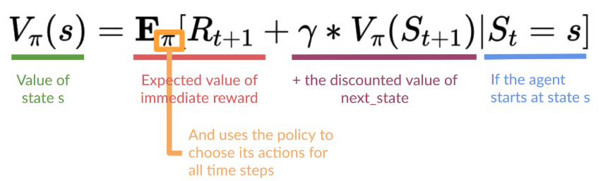
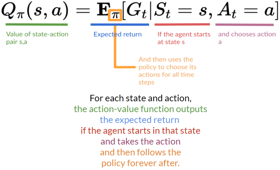
State-Value Functions: denoted as \(V_\pi(s)\), represents the expected cumulative future rewards starting from a particular state \(s\) and following a specific policy \(\pi\) thereafter. It measures the "goodness" of being in the state \(s\), considering the long-term rewards achievable from that state under policy \(\pi\). It does not depend on specific actions but rather on the overall behavior dictated by the policy. \[ \begin{aligned} V_\pi(s)= E_\pi[G_t|S_t=s], \\ \space G_t=\sum^\infty_{k=0}\gamma^kR_{t+k+1} \end{aligned} \] Action-Value Functions: denoted as \(Q_\pi(s,a)\), represents the expected cumulative future rewards starting from the state \(s\), taking action \(a\), and then following a specific policy \(\pi\) thereafter. It measures the “goodness” of taking action \(a\) in state \(s\), considering both immediate rewards and future rewards achievable under the policy \(\pi\). It provides more granular information than \(V(s)\), as it evaluates specific actions rather than just states. \[ Q_\pi(s,a) = E_\pi[G_t|S_t=s, A_t=a] \] The relationship between the state-value function and the action-value function can be expressed using the following formula: \[ V_\pi(s) =\sum_{a \in A} \pi(a|s) Q_\pi (s,a) \] This equation shows that the value of a state under policy \(\pi\), \(V_\pi(s)\), is the expected value of the action-value function \(Q_\pi(s,a)\), weighted by the probability of taking each action \(a\) in state \(s\) according to policy \(\pi(a|s)\).

State-Value Bellman Equation and Action-Value Bellman Equation

State-Value Bellman Equation:

bellman_equation_huggingface

(Source: The Bellman Equation: simplify our value estimation)

The State-Value Bellman Equation can be written in a recursive form. \[ \begin{aligned} V_\pi(s) &= E_\pi(G_t|S_t=s)\\ &= E_\pi(R_{t+1}+rG_{t+1}|S_t=s)\\ &=\sum_a \pi(a|s) \sum_{s'}\sum_r p(s',r|s,a) [r + V_\pi(s')] \end{aligned} \]

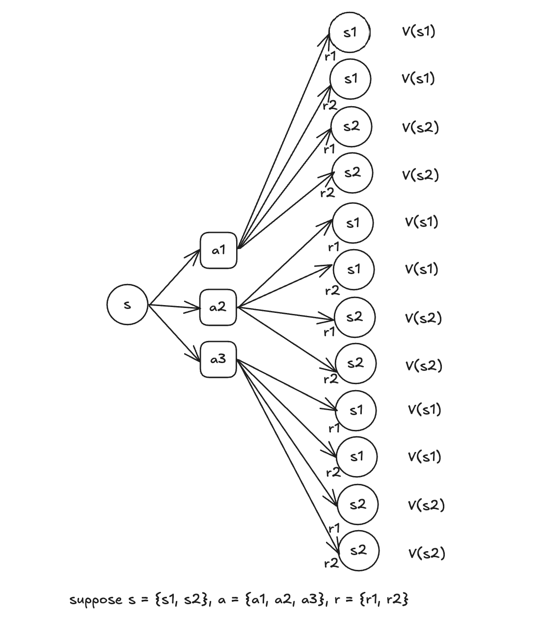
The tree structure below as an example can help understand the recursive property of the State-Value Bellman Equation. Note that an action \(a\) does not necessarily lead to a specific state \(s\), it can result in multiple possible states, each with a certain probability. These probabilities are determined by the environment, which we typically do not have direct access to.

bellman_equation_tree

Action-Value Bellman Equation:

action_value_equation_huggingface

(Source: Two types of value-based methods)

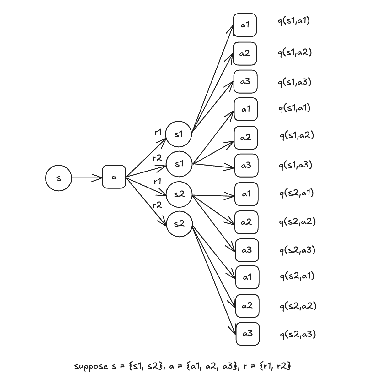
The Action-Value Bellman Equation can be written in a recursive form as well: \[ \begin{aligned} Q_\pi(s,a)&= E_\pi[G_t|S_t=s, A_t=a]\\ &=\sum_{s'}\sum_{r} P(s',r|s,a)[r+\gamma\sum_{a'}\pi(a'|s')Q_\pi(s',a')] \end{aligned} \] The tree structure below as an example can help understand the recursive property of the Action-Value Bellman Equation.

action_value_bellman_equation_tree

The main limitations of Bellman Equation:

• In real-world problems, the number of states can be extremely large, requiring a separate Bellman equation for each state. This results in a system of simultaneous nonlinear equations due to the presence of the max operator, which can be difficult to solve.
• Solving Bellman equations often requires iterative methods and can demand significant computational resources. This is particularly true when seeking high-precision approximations over many iterations.
• In applications like the Bellman-Ford algorithm for finding shortest paths, the presence of negative cycles can pose a problem. If a cycle has a negative total sum of edges, it can lead to an undefined shortest path since iterating through the cycle can indefinitely reduce the path length.
• The Bellman equation is inherently nonlinear because it involves maximizing over possible actions. This nonlinearity can complicate finding solutions, especially when dealing with large state spaces or complex reward structures.

Policy Iteration

In RL, an optimal policy is a policy that maximizes the expected cumulative reward (or return) for an agent across all states in a Markov Decision Process (MDP). This means that the state-value function \(v_{\pi}(s)\) or the action-value function \(q_{\pi}(s,a)\) under the optimal policy is greater than or equal to that of any other policy for all states and actions. \[ \pi^*(s) \geq \pi(s), \forall s \in \text{states} \] In finite MDPs, at least one optimal policy always exists. However, there may be multiple optimal policies that achieve the same maximum expected return.

Policy Iteration is a dynamic programming algorithm used in RL to compute the optimal policy \(\pi^*\) for a Markov Decision Process (MDP). It alternates between two main steps: policy evaluation and policy improvement, iteratively refining the policy until convergence.

The full policy iteration algorithm pseudocode is in the figure below (Source: Sutton & Barto summary chap 04 - Dynamic Programming):

policy_iteration_pseudocode

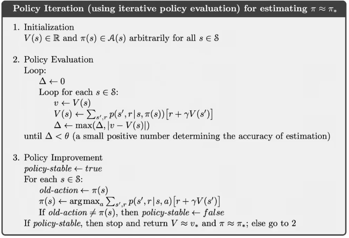
Here is a detailed explanation of this policy iteration's algorithm pseudocode.

Repeat steps until convergence:

1. Policy evaluation: keep current policy \(\pi\) fixed, find value function \(V(\cdot)\).

   Iterate Bellman update until values converge:

   \[ V(s) \leftarrow \sum_{s',r}p(s',r|s,\pi(s))[r+\gamma V(s')] \] The Bellman operator computes future rewards but discounts them by multiplying with \(\gamma\). This ensures that differences in value functions become smaller with each iteration. In other words, Bellman shrinks distances. To see it mathematically,

   The Bellman operator for the state-value function under a fixed policy \(\pi\) is defined as \[ V^{\pi}(s) = r(s, \pi(s)) + \gamma \sum_s P(s|s,\pi(s))V(s') \] This operator updates the value function by combining the immediate reward and the discounted future rewards.

   We compute the difference after applying the operator: \[ \Big|V^{\pi}_1(s)-V^{\pi}_2(s)\Big| = \Big|r(s,\pi(s))+\gamma\sum_s P (s|s,\pi(s))V_1(s')-\Big[r(s,\pi(s))+\gamma\sum_s P (s|s,\pi(s))V_2(s')\Big]\Big| \] Simplify by canceling out the immediate rewards, we get: \[ \Big|V^{\pi}_1(s)-V^{\pi}_2(s)\Big| = \gamma \Big|\sum_s P (s|s,\pi(s))\Big(V_1(s')-V_2(s')\Big)\Big| \] Since \(\gamma<1\), the difference between \(V_1^{\pi}(s)\) and \(V_1^{\pi}(s)\) is always smaller than the difference between \(V_1(s')\) and \(V_1(s')\). Because Bellman operator shrinks distances, it is a contraction mapping and follows the contraction mapping property.

   In summary, Policy evaluation is a contraction mapping for a fixed policy \(\pi\). Policy evaluation converges because it applies a contraction mapping repeatedly to compute the value function for a fixed policy.

2. Policy improvement: find the best action for \(V(\cdot)\) via one-step lookahead.

   During policy improvement, the current policy \(\pi\) is updated by selecting actions that maximize the expected return for each state \(s\).

   \(\pi(s) \leftarrow \arg \max_a \sum_{s',r}p(s',r|s,a)[r+\gamma V(s')]\)

   The intuition behind: \(V^{\pi}(s)\) measures how good it is to start from the state \(s\) and follow policy \(\pi\). By improving the actions selected by the policy, we ensure that the agent transits into states with higher expected cumulative rewards. This iterative process ensures that each new policy improves upon or equals the previous one in terms of total expected rewards.

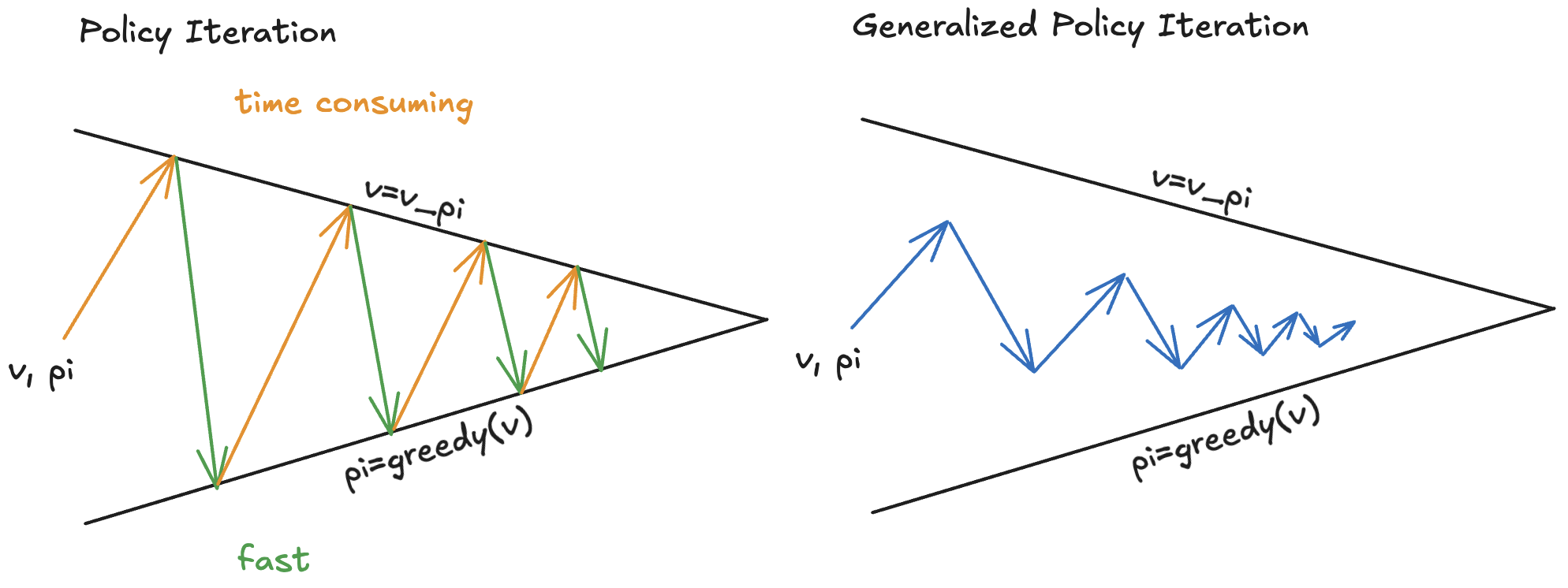
Overall, the idea of Policy Iteration can be demonstrated in the diagram below. The evaluation process usually takes a long time while the improvement process is usually fast.

policy_iteration_eval_impro_demo

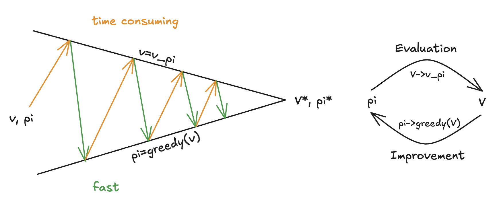
The Generalized Policy Iteration (GPI) method can speed up the policy evaluation process. In GPI, policy evaluation process can be approximate or partial (e.g., only a few iterations instead of full convergence). Policy improvement can also be done incrementally or partially. GPI speeds up the process of finding an optimal policy by relaxing the strict requirements of full convergence in policy evaluation.

generalized_policy_iteration

Monte Carlo Method

Monte Carlo methods are specifically designed for episodic tasks, where each episode eventually terminates, regardless of the actions taken by the agent. An episode refers to a complete sequence of interactions between an agent and the environment, starting from an initial state and ending in a terminal state.

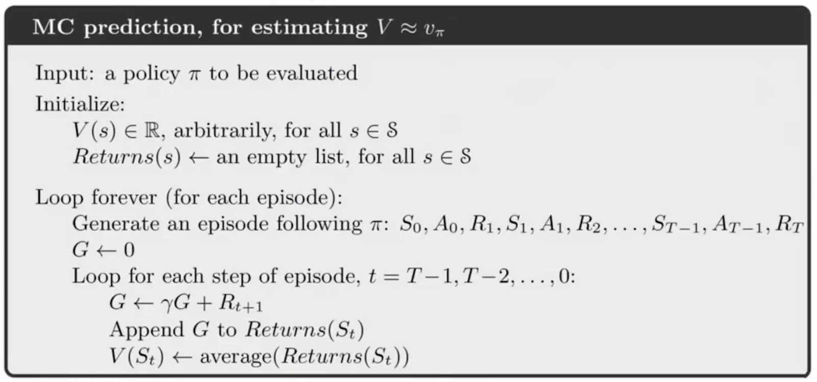
Monte Carlo for Policy Evaluation

Value function and policy updates occur only after an episode is complete. By waiting for the end of an episode, Monte Carlo methods ensure that all rewards following a state are included in the return calculation. Monte Carlo methods learn purely from sampled experience (episodes), without requiring knowledge of transition probabilities or reward models. Episodes allow Monte Carlo methods to handle stochastic environments by averaging returns across multiple episodes.

Here is an example of calculating the state-value functions and action-action functions by Monte Carlo Method once 2 episodes are completed. Given states \(S=[A,B,C,D,E], A=[1,2,3]\), and two episodes \(E_1,E_2\), (Note: \(A:(1,0.4)\) means state \(A\), action \(1\), and reward \(0.4\)) \[ \begin{aligned} &E_1 = \{A:(1,0.4), B:(2,0.5), A:(2,0.6), C:(2,0.1), B:(3,0.8), E:()\}\\ &E_2 = \{B:(2,0.5), A:(1,0.6), C:(2,0.3), A:(1,0.3), C:(2,0.8), E:()\} \end{aligned} \]

1. State-Value Functions Calculation

   We can calculate \(V(A),V(B),V(C),V(D),V(E)\).

   e.g. there are 4 sequences starting from state \(A\), then the state value function is: \[ \begin{aligned} V(A) &= [(0.4+\gamma 0.5 + \gamma^2 0.6 + \gamma^3 0.1 + \gamma^4 0.8)\\ &+(0.6+\gamma 0.1 + \gamma^2 0.8)\\ &+(0.6+\gamma 0.3 + \gamma^2 0.3 + \gamma^4 0.8)\\ &+(0.3+\gamma 0.8)] / 4 \end{aligned} \]

2. Action-Value Functions Calculation

   We can calculate \(Q(A,1),Q(B,2),\cdots\).

   e.g. there are three sequences starting from \(A:(1,)\), then the action value function is \[ \begin{aligned} Q(A,1) &= [(0.4+\gamma 0.5 + \gamma 0.6 + \gamma^3 0.1+ \gamma^4 0.8)\\ &+(0.6+\gamma 0.3 + \gamma^2 0.3 + \gamma^3 0.8)\\ &+(0.3+\gamma 0.8)]/3 \end{aligned} \]

The pseudocode for the above Monte Carlo for Policy Evaluation is as follows (Source: Reinforcement Learning by Sutton and Barto, Chapter 5):

montecarlo_statevalue

As part of the algorithm, it loops for each step of episode from the end \(T-1\) to the beginning of the episode. This allows for dynamic programming where some values can be stored and do not need to be re-calculated (see a simple demonstration below).

montecarlo_algo_dynamic_program

Monte Carlo for Policy Improvement

\[ \pi_{k+1}(s)=\arg \max_a q_{\pi_k}(s,a) \]

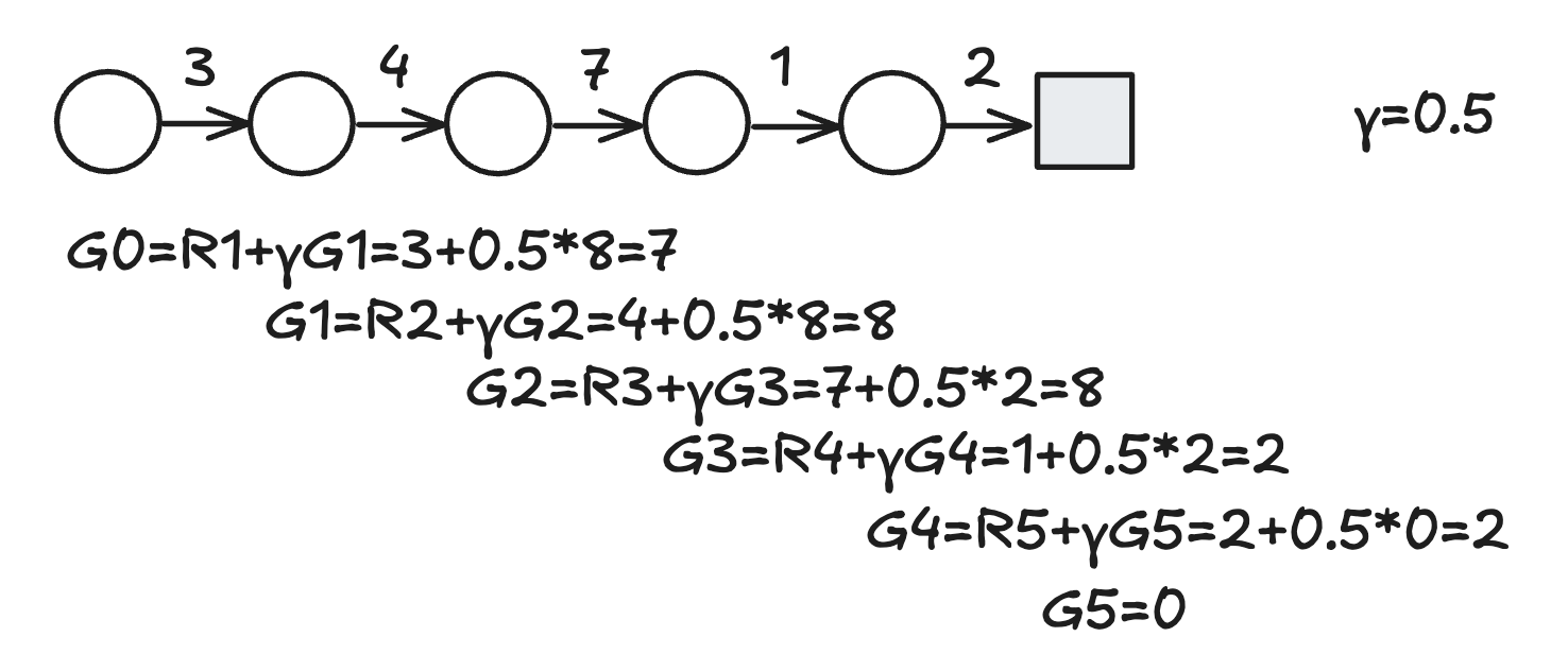
Here is an example of updating policy by action-value function. Given states \(S=[A,B,C,D,E], A=[1,2,3], \gamma=0.5\), and a episode \(E\), (Note: \(A:(1,0.7)\) means state \(A\), action \(1\), and reward \(0.7\)) \[ E = \{A:(1,0.7), B:(1,0.4), A:(3,1.5), C:(2,0.1), B:(3,0.7), A:(1,0.3)\}\ \] Through dynamic programming, cumulative reward is \(G_5(A,1)=0.3\), \(G_4(B,3)=0.7+0.5*3=0.85\), \(G_3(C,2)=0.1+0.5*0.85=0.52\), \(G_2(A,3)=1.5+0.52*0.5=1.76\), \(G_1(B,1)=0.4+1.76*0.5=1.28\), \(G_0(A,1)=0.7+1.28*0.5=1.34\). We can maintain three lists to make the algorithm work:

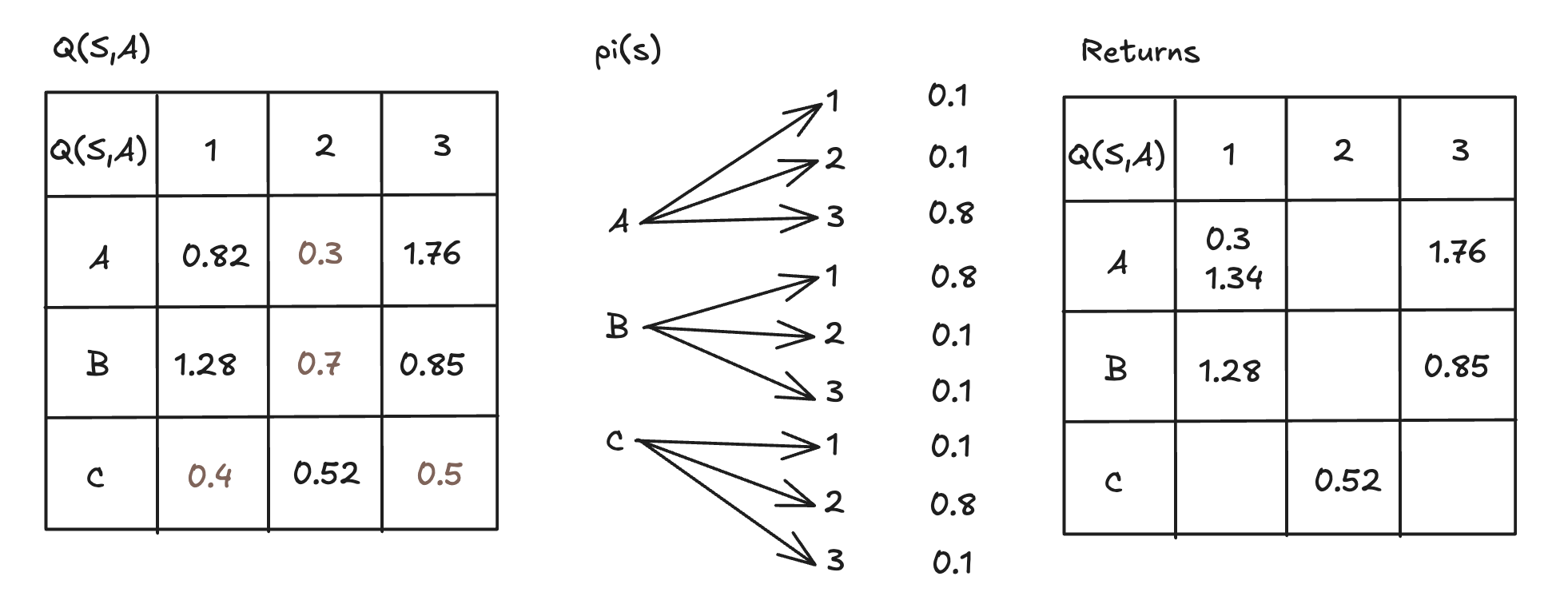
• Return matrix \(Returns(S,A)\), dimension \((S, A)\): It stores cumulative reward values \(G(S=s,A=a)\). One cell can store multiple values as the number of episodes increases.
• \(Q(S,A)\) matrix: It's initialized as random numbers at the beginning. Updated whenever the return matrix is updated. \(Q(S,A)\) is the average value of the corresponding \(Returns(S,A)\).
• \(\pi(s)\) list: It's updating Epsilon values by giving \(1-\epsilon\) probability to the action with highest reward for each state, according to the updated \(Q(S,A)\) matrix. It facilitates Epsilon Greedy Algorithm.

The final updating result of the above example is in the diagram below.

mc_action_value_update_res

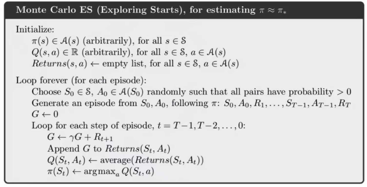
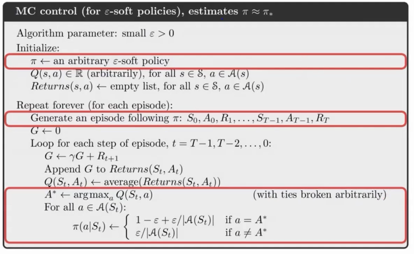
The pseudocode for the above Monte Carlo for Policy Improvement with action-value function is as follows (Source: Reinforcement Learning by Sutton and Barto, Chapter 5):

monte_carlo_action_value

mc_control_epsilon_pi

Main Limitation

• Policy updates occur only after an episode is completed, which can slow down learning compared to methods like Temporal Difference (TD) learning that update incrementally after each step.
• MC methods do not use bootstrapping (i.e., they do not update value estimates based on other estimates). While this avoids bias, it also means MC methods cannot leverage intermediate value estimates, leading to slower convergence.

Temporal Difference Learning

TD leanring focuses on estimating the value function of a given policy by updating value estimates based on the difference between successive predictions, rather than waiting for an entire episode to conclude.

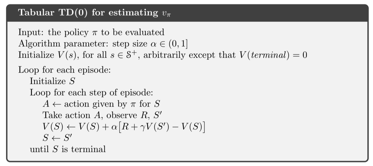
Given \[ \begin{aligned} V(S_t) &\leftarrow V(S_t) + \alpha \Big[G_t - V(S_t)\Big]\\ G_t &= R_{t+1} + \gamma R_{t+2} + \gamma^2 R_{t+3} + ... = R_{t+1} + \gamma G_{t+1}\\ V_{\pi}(s) &= E_\pi[G_t|S_t=s] = E_\pi\Big[R_{t+1} + \gamma G_{t+1}| S_t=s\Big] = R_{t+1} + \gamma V_\pi(S_{t+1}) \end{aligned} \] We can derive the core function of TD: \[ V(S_t) \leftarrow V(S_t) + \alpha [R_{t+1} + \gamma V(R_{t+1}) - V(S_t)] \] The pseudocode of TD learning is as follows. (Source: Sutton & Barto summary chap 06 - Temporal Difference Learning)

td_learning_for_v

From table to function approximation

Main limitations of table based methods:

• As the number of state variables increases, the size of the state space grows exponentially.
• Storing a value table becomes impractical for large or continuous state/action spaces due to memory limitations.
• Table-based methods treat each state (or state-action pair) independently. They cannot generalize knowledge from one part of the state space to another, requiring every state to be visited multiple times for accurate learning.
• In large state spaces, it is unlikely that an agent will visit all relevant states/actions frequently enough to converge to an optimal policy within a reasonable time frame.
• Table-based methods are well-suited for small problems but fail to scale to real-world applications such as autonomous driving, robotics, or complex games like Go or StarCraft.

From tabular to parametric functions:

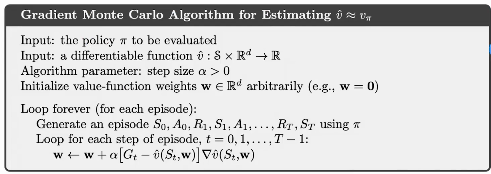
Fit a parametric function to approximate the value function \(V(s)\) which maps states \(s\) to their corresponding value estimates. \[ f(s,\theta) \approx V(s) \] where \[ f(s,\theta)=w^Ts+b \] To optimize this approximation, we minimize the mean squared error (MSE) loss between the observed value \(v(s)\) and predicted \(\hat{v}(s,{w})\) from Monte Carlo. \(\mu(s)\) is the probability distribution over states. This loss ensures that the predicted values are as close as possible to the observed values. \[ \ell = \min \sum_s \mu(s) \Big[v_\pi(s)-\hat{v}(s,{w})\Big]^2 \] The optimal \({w}\) that minimize the loss can be found by batch Gradient Descent (\(\eta\) is learning rate). \[ w \leftarrow w - \eta \nabla \ell(w) \] where \[ \begin{aligned} \nabla \ell(w) &= \nabla \sum_s \mu(s) \Big[v_\pi(s) - \hat{v}(s,{w})\Big]^2\\ &= \sum_s \mu(s) \nabla \Big[v_\pi(s) - \hat{v}(s,{w})\Big]^2\\ &= -2 \sum_s \mu(s) \Big[v_\pi(s) - \hat{v}(s,{w})\Big]\nabla \hat{v}(s,{w}) \end{aligned} \] From Gradient Descent to Stochastic Gradient Descent:

While batch gradient descent computes gradients over the entire dataset (all states), this can be computationally expensive for large-scale problems. Instead, stochastic gradient descent (SGD) updates the parameters incrementally using one observation at a time. Given observations \((S_1, v_\pi(S_1)), (S_2, v_\pi(S_2)), (S_3, v_\pi(S_3)), ...\), SGD performs updates as follows (\(\alpha\) is learning rate). \[ \begin{aligned} {w}_2 &= {w}_1 + \alpha \Big[v_\pi(S_1) - \hat{v}(S_1,{w_1})\Big] \nabla \hat{v}(S_1,{w}_1)\\ {w}_3 &= {w}_2 + \alpha \Big[v_\pi(S_2) - \hat{v}(S_2,{w_2})\Big] \nabla \hat{v}(S_2,{w}_2)\\ &\cdots \end{aligned} \] The algorithm of Gradient Monte Carlo is as follows. (Source: Reinforcement Learning by Sutton and Barto)

gradient_montecarlo_v

PPO Prior

Average Reward

The average reward is an alternative to the commonly used discounted reward framework. It measures the long-term average reward per time step under a given policy, making it particularly suitable for continuing tasks (non-episodic problems) where there is no natural endpoint or terminal state.

The average reward framework is particularly useful for continuing tasks, where:

• The task does not have a natural termination point (e.g., robot navigation, server optimization, or industrial control systems).
• The agent operates indefinitely, and evaluating its performance based on long-term behavior (rather than episodic returns) is more meaningful.

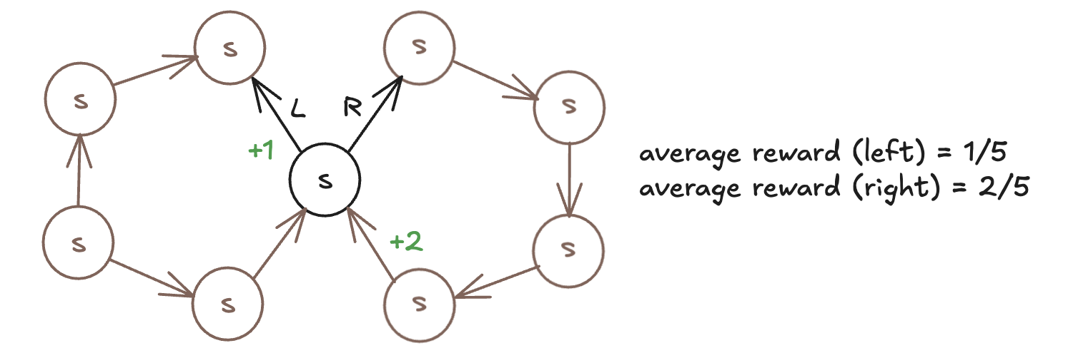
The average reward for a policy is defined as: \[ r(\pi)=\lim_{h \rightarrow \infty} {1\over h}\sum^h_{t=1} E\Big[R_t | S_0, A_{0:t-1} \sim \pi\Big] \] This simple example shows how average reward is calculated:

average_reward_policy

Differential Return

The differential return in RL is a concept that arises in the average reward framework, particularly for continuing tasks. It measures the cumulative deviation of rewards from the long-term average reward rate, \(r(\pi)\) , under a given policy \(\pi\).

Differential return aligns with the goal of maximizing long-term performance in continuing tasks by focusing on deviations from steady-state behavior. Unlike discounted returns, differential return does not rely on a discount factor \(\gamma\). This avoids biases introduced by choosing an arbitrary discount factor. It is particularly well-suited for tasks with no natural termination, such as robotics or industrial control systems.

The differential return at time step \(t\) is defined as: \[ G_t = R_{t+1} - r(\pi)+R_{t+2} - r(\pi)+R_{t+3} - r(\pi) \] Then the value functions can be rewritten as \[ \begin{aligned} v_\pi(s) = \sum_a \pi(a|s)\sum_{r,s'} p(s',r|s,a) \Big[r-r(\pi) +v_{\pi}(s')\Big]\\ q_\pi(s,a) = \sum_{r,s'} p(s',r|s,a) \Big[r-r(\pi) +\sum_{a'}\pi(a'|s')q_{\pi}(s',a')\Big] \end{aligned} \] Algorithms like Gradient Monte Carlos can be rewritten by using this differential return.

Policy Gradient and REINFORCE

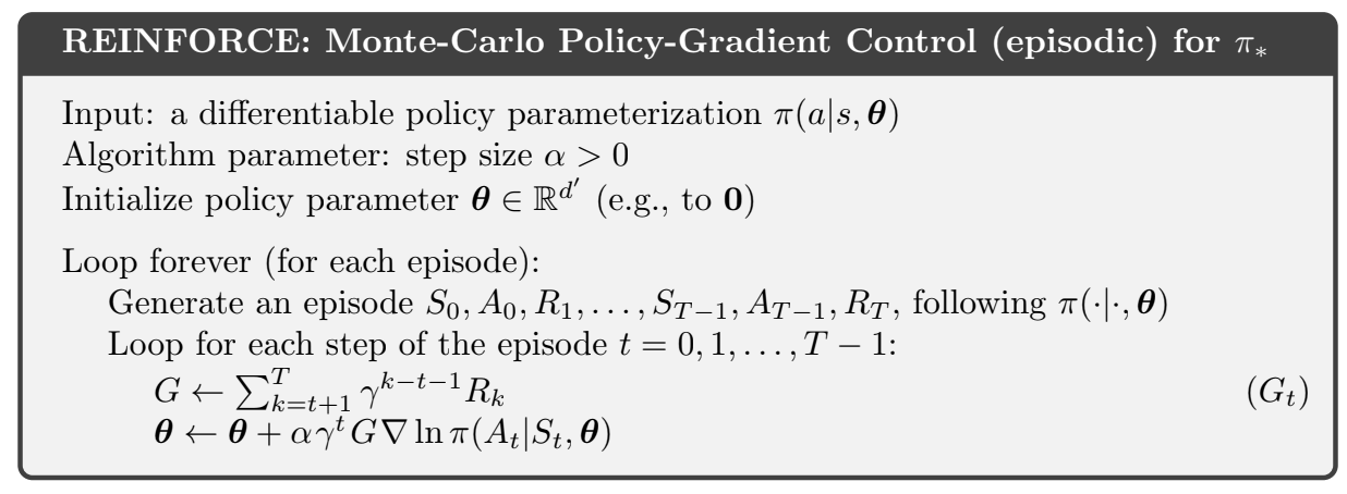
Objective of policy gradient: \[ \begin{aligned} J(\theta) &= \sum_{s\in S}d^{\pi}(s)V^\pi(s) = \sum_{s\in S} d^\pi(s) \sum_{a\in A} \pi_\theta(a|s) Q^\pi(s,a)\\ d^\pi(s) &= \lim_{t\rightarrow \infty}P(s_t=s|s_o,\pi_\theta) \rightarrow \text{ converege (Markov Property)}\\ &\max J(\theta): \\ &\max \sum_{s\in S} d^\pi(s) V^\pi(s) \implies \theta \leftarrow \theta + \nabla_\theta J(\theta) \end{aligned} \] Policy gradient theorem allows us to compute the gradient of the expected return with respect to the parameters of a parameterized policy, enabling optimization through gradient ascent. \[ \begin{aligned} \nabla_\theta J(\theta) &= \nabla _\theta\Big[\sum_{s\in S} d^\pi(s) \sum_{a\in A} \pi_\theta(a|s) Q^\pi(s,a)\Big]\\ &\propto \sum_{s\in S} d^\pi(s) \sum_{a\in A} Q^\pi(s,a) \nabla _\theta\pi_\theta(a|s)\\ &\implies \theta \leftarrow \theta + \eta\Big[\sum_{s\in S} d^\pi(s) \sum_{a\in A} Q^\pi(s,a) \nabla _\theta\pi_\theta(a|s) \Big] \end{aligned} \] Since Monte Carlo involves a sampling step, which requires an expectation form. The gradient derived above can be re-written as follows, supporting gradient estimation. (Recall: \((\ln x)' = 1/x\)) \[ \begin{aligned} \nabla_\theta J(\theta) &\propto \sum_{s\in S} d^\pi(s) \sum_{a\in A} Q^\pi(s,a) \nabla _\theta\pi_\theta(a|s)\\ &=\sum_{s\in S}d^\pi(s) \sum_{a\in A} \pi_\theta(a|s) Q^\pi(s,a) {\nabla_{\theta} \pi_\theta(a|s)\over \pi_\theta(a|s)}\\ &=E_\pi\Big[Q^\pi(s,a)\nabla_\theta \ln\pi_\theta(a|s)\Big]\\ (&=E_{s \sim \pi, a \sim \pi_\theta(a|s)}\Big[Q^\pi(s,a)\nabla_\theta \ln\pi_\theta(a|s)\Big])\\ \end{aligned} \] Given the above theorems, a Reinforce Algorithm - Monte-Carlo Policy-Gradient algorithm is defined as follows. (Source: Sutton & Barto summary chap 13 - Policy Gradient Methods)

montecarlo_policy_gradient_pi

A differentiable policy ensures that small changes in \(\theta\) result in smooth changes in the action probabilities \(\pi(a|s,\theta)\). This is crucial for stable and efficient learning. The softmax function is commonly used to parameterize policies in discrete action spaces. The softmax function is smooth and differentiable, enabling gradient-based optimization. Softmax ensures that all actions have non-zero probabilities, promoting exploration during training.

Here the differentiable policy parameterization \(\pi(a|s,{\theta})\) can be defined by \[ \pi(a|s,\theta) = {\exp(h(s,a,\theta)) \over \sum_{b\in A} \exp(h(s,b,\theta))} \] where \(h(s,a,\theta)=w_a^T+b_a\) is a linear or non-linear function representing the preference for action \(a\). The denominator normalizes the probabilities so that they sum to 1.

The log of the softmax function has a convenient derivative that simplifies gradient computation: \[ \nabla_\theta\ln \pi(a,s,\theta) = \nabla_\theta h(s,a,\theta) - \sum_b \pi(b|s,\theta) \nabla_\theta h(s,b,\theta) \]

Main Limitations of REINFORCE

• REINFORCE requires complete episodes to compute the return for each state, as it relies on Monte Carlo estimates of the expected return. This makes it unsuitable for continuing tasks (non-episodic environments) where there is no clear terminal state.
• The gradient estimates in REINFORCE have high variance because they depend on the total return from sampled episodes, which can vary significantly due to stochasticity in the environment and policy.
• Since REINFORCE updates the policy only after completing an episode, it does not make use of intermediate data. This results in poor sample efficiency, requiring a large number of episodes to learn effectively.
• Unlike Temporal Difference (TD) methods, REINFORCE does not use bootstrapping (i.e., it does not update value estimates based on other estimates). It relies solely on complete returns from episodes.
• The algorithm is highly sensitive to the choice of the learning rate. A poorly chosen learning rate can lead to divergence or extremely slow convergence.

Advantage Function

Advantage function employs the idea of differential return. In the REINFORCE algorithm, with advantage function, policy gradient can be re-written as \[ \begin{aligned} \nabla_\theta J(\theta) &=E_\pi\Big[Q^\pi(s,a)\nabla_\theta \ln\pi_\theta(a|s)\Big]\\ &=E_\pi\Big[A^\pi(s,a)\nabla_\theta \ln\pi_\theta(a|s)\Big]\\ \end{aligned} \] where \[ \begin{aligned} A^{\pi}(s,a) &= Q^\pi(s,a)-V^\pi(s)\\ V^\pi(s) &= \sum_{a\in A}\pi(a|s) Q(s,a) \end{aligned} \]

Off-Policy Policy Gradient

Off-policy policy gradient methods allow learning a target policy while using data generated from a different behavior policy. By reusing past experiences and learning from suboptimal actions, off-policy methods can significantly improve sample efficiency. Off-policy learning allows for better exploration strategies since it can incorporate data from various policies, including exploratory ones.

The policy gradient estimate is defined as \[ \nabla_\theta J(\theta) = E_\beta\Big[{\pi_\theta(a|s)\over \beta(a|s)} Q^\pi(s,a) \nabla _\theta \ln \pi_\theta (a|s)\Big] \] \(\beta(a|s)\) refers to the behavior policy that generates the data used for training. The behavior policy is not necessarily the optimal policy we want to learn (the target policy \(\pi(a|s)\)). Instead, it can be any policy that provides useful exploration of the state-action space. \({\pi_\theta(a|s)\over \beta(a|s)}\) is the important weight for sampling.

Trust Region Policy Optimization (TRPO)

TRPO is an advanced policy gradient method in RL designed to optimize policies while ensuring stable and reliable updates. It addresses some of the limitations of traditional policy gradient methods by incorporating a trust region constraint that limits how much the policy can change in a single update. The difference between REINFORCE and TRPO is that TRPO uses off-policy policy gradient and advantage function, as well as a constraint on the Jullback-Leibler (KL) divergence between the old and new policy.

Recall that REINFORCE's objective of policy gradient is: \[ J(\theta) = \sum_{s\in S} d^\pi(s) \sum_{a\in A} \pi_\theta(a|s) Q^\pi(s,a) \] The derivation of TRPO's objective of policy gradient is: \[ \begin{aligned} J(\theta) &=\sum_{s \in S} d^{\pi}(s) \sum_{a\in A} (\pi_\theta(a|s) \hat{A}_{\theta_{old}}(s,a))\\ &=\sum_{s\in S} d^{\pi_{\theta_{old}}} \sum_{a\in A} (\beta(a|s) {\pi_\theta(a|s)\over \beta(a|s)} \hat{A}_{\theta_{old}}(s,a))\\ &=E_{s\sim d^{\pi_{\theta_{old}}}, a \sim \beta}\Big[{\pi_\theta(a|s)\over \beta(a|s)} \hat{A}_{\theta_{old}}(s,a)\Big]\\ &=E_{s\sim d^{\pi_{\theta_{old}}}, a \sim \pi_{\theta_{old}}}\Big[{\pi_\theta(a|s)\over \pi_{\theta_{old}}(a|s)} \hat{A}_{\theta_{old}}(s,a)\Big]\\ E_{s\sim d^{\pi_{\theta_{old}}}}&\Big[D_{KL}\Big(\pi_{\theta_{old}}(\cdot | s)||\pi_\theta(\cdot|s)\Big)\Big] \leq \delta \end{aligned} \] The TRPO constrained optimization is defined as \[ \begin{aligned} &\max E_{s\sim d^{\pi_{\theta_{old}}}, a \sim \pi_{\theta_{old}}}\Big[{\pi_\theta(a|s)\over \pi_{\theta_{old}}(a|s)} \hat{A}_{\theta_{old}}(s,a)\Big]\\ & s.t. E_{s\sim d^{\pi_{\theta_{old}}}}\Big[D_{KL}\Big(\pi_{\theta_{old}}(\cdot | s)||\pi_\theta(\cdot|s)\Big)\Big] \leq \delta \end{aligned} \] One of the main limitations of TRPO is that the constrained optimization problem can be computationally intensive, especially for large state and action spaces.

PPO

PPO Objective

To address the computational expense of the constrained optimization in TRPO, researchers introduced the CLIP objective in policy gradient methods. The CLIP objective simplifies the optimization process while maintaining stable policy updates. Below are the TRPO objective and its corresponding CLIP version: \[ \begin{aligned} J^{TRPO}(\theta) &= E[r(\theta)\hat{A}_{\theta_{old}}(s,a)]\\ J^{CLIP}(\theta) &= E[\min(r(\theta)\hat{A}_{\theta_{old}}(s,a)), \text{clip}(r(\theta),1-\epsilon, 1+\epsilon) \hat{A}_{\theta_{old}}(s,a)] \end{aligned} \] where \[ \begin{aligned} &r(\theta) = {\pi_{\theta (a|s)} \over \pi_{\theta_{old}(a|s)}}\\ &r(\theta) \in [1-\epsilon, 1+ \epsilon], \\ &i.e. 1-\epsilon \leq r(\theta) \leq 1+\epsilon \end{aligned} \] If \(r(\theta) > 1+\epsilon, r(\theta)=1+\epsilon\). If \(r(\theta) < 1-\epsilon, r(\theta) = 1-\epsilon\).

The CLIP objective ensures that the policy ratio \(r(\theta)\) does not deviate too far from 1 (the old policy), thereby limiting large updates to the policy. The term \(J^{CLIP}(\theta)\) takes the minimum of the “unclipped” objective and the “clipped” version. This prevents overly large policy updates by removing the lower bound when \(r(\theta)\) is outside the clipping range.

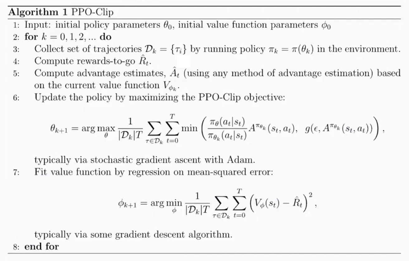
The Proximal Policy Optimization (PPO) algorithm (Paper: Proximal Policy Optimization Algorithms) extends the CLIP objective by incorporating additional terms for value function optimization and entropy regularization. The full PPO objective is defined as: \[ J^{PPO}(\theta) = E[J^{CLIP}(\theta) - c_1(V_\theta(s)-V_{target})^2 + c_2 H(s,\pi_\theta(\cdot))] \] where

• \(-(V_\theta(s) - V_{target})^2\) is the negative mean squared error (MSE), which we aim to maximize. It minimizes the difference between the predicted value function \(V_\theta(s)\) and the target value \(V_{target}\). The coefficient \(c_2\) controls the tradeoff between policy optimization and value function fitting.
• \(H(s,\pi_\theta(\cdot))\) represents the entropy of the policy. Maximizing entropy encourages exploration by preventing premature convergence to deterministic policies. The coefficient \(c_2\) determines the weight of this entropy term.

Here is a pseudocode of PPO-Clip Algorithm (Source: OpenAI Spinning Up - Proximal Policy Optimization)

ppo_clip_algo

PPO Usage

State, Action, and Reward in the Context of LLMs

In the context of LLMs, the components of reinforcement learning are defined as follows:

1. State: The state corresponds to the input prompt or context provided to the language model. It represents the scenario or query that requires a response.
2. Action: The action is the output generated by the language model, i.e., the response or continuation of text based on the given state (prompt).
3. Reward: The reward is a scalar value that quantifies how well the generated response aligns with human preferences or task objectives. It is typically derived from a reward model trained on human feedback.
4. Policy: A policy refers to the strategy or function that maps a given state (input prompt and context) to an action (the next token or sequence of tokens to generate). The policy governs how the LLM generates responses and is optimized to maximize a reward signal, such as alignment with human preferences or task-specific objectives.

Steps of RLHF Using PPO

The RLHF process using PPO involves three main stages:

1. Training a Reward Model: A reward model is trained to predict human preferences based on labeled data. Human annotators rank multiple responses for each prompt, and this ranking data is used to train the reward model in a supervised manner. The reward model learns to assign higher scores to responses that align better with human preferences.

2. Fine-Tuning the LLM with PPO: After training the reward model, PPO is used to fine-tune the LLM. The steps are as follows:

   1. Initialize Policies: Start with a pre-trained LLM as both the policy model (actor) and optionally as the critic for value estimation.

      • The actor is the language model that generates responses (actions) based on input prompts (states).

        For example: Input: “Explain quantum mechanics.” Output: “Quantum mechanics is a branch of physics that studies particles at atomic and subatomic scales.”

      • The critic is typically implemented as a value function, which predicts how good a particular response (action) is in terms of achieving long-term objectives. This model predicts a scalar value for each token or sequence, representing its expected reward or usefulness.

        For example:

        Input: “Explain quantum mechanics.” → “Quantum mechanics is…” Output: A value score indicating how well this response aligns with human preferences or task objectives.

      • Both the actor and critic can be initialized from the same pre-trained LLM weights to leverage shared knowledge from pretraining. However, their roles diverge during fine-tuning: The actor focuses on generating responses. The critic focuses on evaluating those responses.

   2. Collect Rollouts: Interact with the environment by sampling prompts from a dataset. Generate responses (actions) using the current policy. Compute rewards for these responses using the trained reward model.

   3. Compute Advantage Estimates: Use rewards from the reward model and value estimates from the critic to compute advantages: \[ \hat{A}(s, a) = R_t + \gamma V(s_{t+1}) - V(s_t), \] where $ R_t $ is the reward from the reward model.

   4. Optimize Policy with PPO Objective: Optimize the policy using PPO's clipped surrogate objective: \[ J^{CLIP}(\theta) = \mathbb{E}\left[\min\left(r(\theta)\hat{A}(s, a), \text{clip}(r(\theta), 1-\epsilon, 1+\epsilon)\hat{A}(s, a)\right)\right], \] where $ r() = $ is the probability ratio between new and old policies.

   5. Update Value Function: Simultaneously update the value function by minimizing mean squared error between predicted values and rewards: \[ \mathcal{L}_{\text{value}} = \mathbb{E}\left[(V_\theta(s) - R_t)^2\right]. \]

   6. Repeat: Iterate over multiple epochs until convergence, ensuring stable updates by clipping policy changes.

3. Evaluation: Evaluate the fine-tuned LLM on unseen prompts to ensure it generates outputs aligned with human preferences. Optionally, collect additional human feedback to further refine both the reward model and policy.

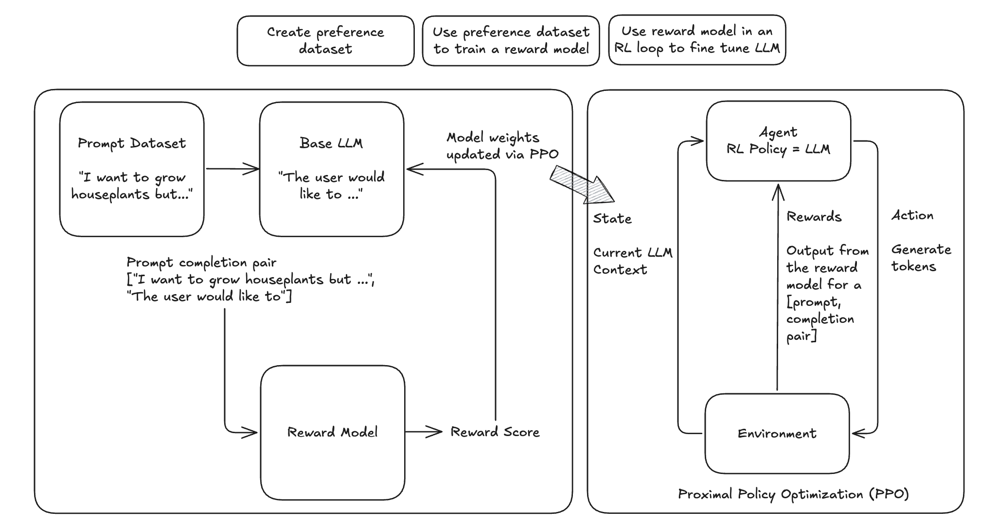
The following diagrams summarizes the high-level RLHF process with PPO, from preference data creation, to training a reward model, and using reward model in an RL loop to fine tune LLM.

PPO_RLHF_flowchart

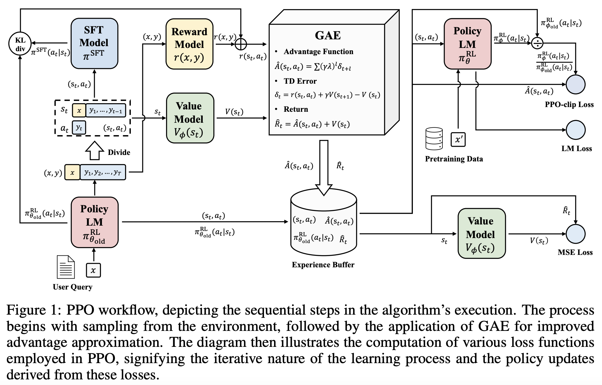
The following workflow chart illustrates the more detailed training process of RLHF with PPO. (Source: Secrets of RLHF in Large Language Models Part I: PPO)

RLHF_training_realworld

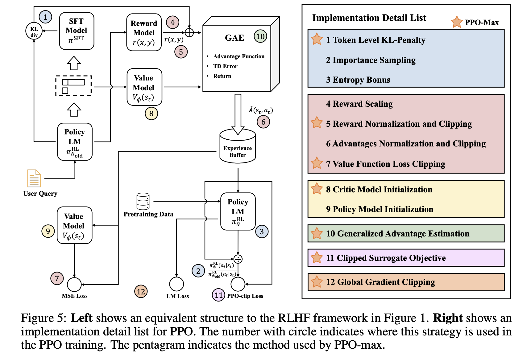
RLHF Training Tricks

There are practical challenges that arise during RLHF training. These challenges stem from the inherent complexities of RL, especially when applied to aligning LLMs with human preferences. Therefore, tricks are essential for addressing the practical limitations of RLHF, ensuring the training process remains efficient, stable, and aligned with human preferences while minimizing the impact of inherent challenges in RL systems. (Source: Secrets of RLHF in Large Language Models Part I: PPO)

RLHF_training_tricks

DPO

Bradley-Terry and Plackett-Luce Reward Model

The Bradley-Terry (BT) model is a probabilistic model used to compare pairwise preferences. It assumes that each item (e.g., a response or completion) has an intrinsic quality score, and the probability of one item being preferred over another depends on the relative difference in their scores.

Mathematically, the probability of option \(y_1\) being preferred over option \(y_2\) is given by: \[ P(y_1 \succ y_2|x) = {\exp(r(x,y_1)) \over \exp(r(x,y_1)) + \exp(r(x,y_2))} \] The loss of this reward model is \[ L_R(r_{\phi},D) = -E_{(x,y_w,y_l)\sim D} \Big[\log \sigma\Big(r_{\phi}(x,y_w) - r_{\phi}(x,y_l)\Big)\Big] \] However, the BT model has some limitations:

• It assumes transitivity in preferences (if \(A>B\) and \(B>C\), then \(A >C\)), which may not always hold in real-world data.
• It only handles pairwise comparisons and does not naturally extend to rankings involving more than two items.

The Plackett-Luce (PL) model generalizes the Bradley-Terry model to handle rankings of multiple items, not just pairwise comparisons. It models the probability of a ranking as a sequence of choices. The first-ranked item is chosen based on its relative worth compared to all other items. The second-ranked item is chosen from the remaining items, and so on.

Mathematically, for a ranking \(i_1\succ i_2 \succ ... \succ i_J\), the probability is given by: \[ P(i_1\succ i_2 \succ ... \succ i_J ) = \prod^j_{j=1}{\alpha_{i_j}\over \sum^J_{k=j} \alpha_{i_k}} \] where \(\alpha_{i_j}\) is the worth or quality score of item \(i_j\). The denominator normalizes over all remaining items at each step.

The PL model has several advantages over the BT model:

• Unlike BT, which only works with pairwise comparisons, PL can handle rankings involving multiple items.
• PL can accommodate partial rankings (e.g., ranking only the top n items), making it more versatile in scenarios where full rankings are unavailable.
• When human feedback involves ranking multiple responses rather than just picking one as better, PL captures this richer information better than BT.

DPO Objective

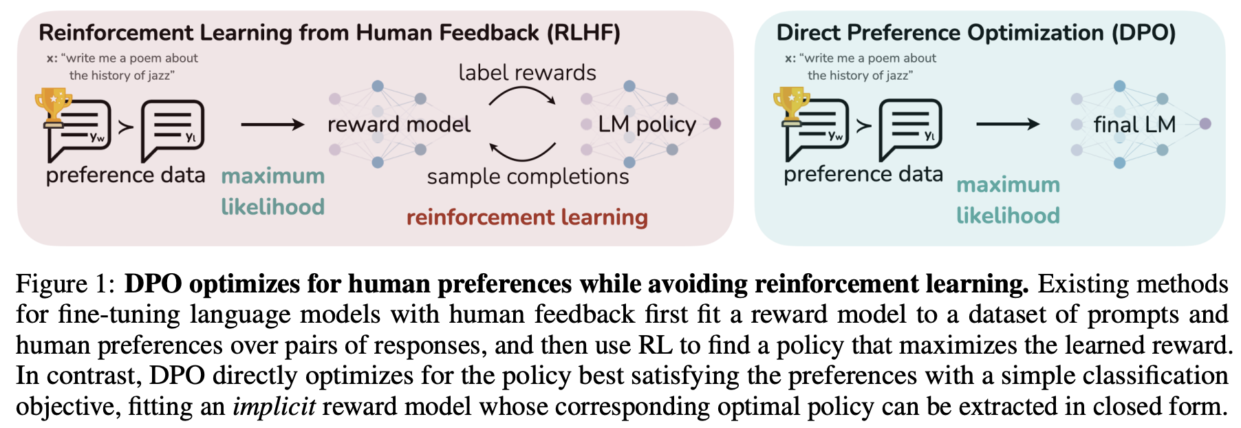
The main reason why RLHF with PPO is hard is that it takes a lot of redundant effort. Policy Model is all we need, all other efforts are not necessary. DPO (Direct Preference Optimization) is a novel alternative to traditional RLHF for fine-tuning LLMs. It simplifies the RLHF process by eliminating the need for complex reward models and RL algorithms. Instead, DPO reframes the problem of aligning LLMs with human preferences as a classification problem using human-labeled preference data.

The idea is DPO and difference between DPO and PPO are shown in the figure below (Source: Direct Preference Optimization: Your Language Model is Secretly a Reward Model)

DPO_idea

Recall the Bradley-Terry reward model: \[ \begin{aligned} P(y_1 \succ y_2|x) &= {\exp(r(x,y_1)) \over \exp(r(x,y_1)) + \exp(r(x,y_2))}\\ L_R(r_{\phi},D) &= -E_{(x,y_w,y_l)\sim D} \Big[\log \sigma\Big(r_{\phi}(x,y_w) - r_{\phi}(x,y_l)\Big)\Big] \end{aligned} \] RLHF objective is defined as follows. Keep in mind that no matter whether DPO or PPO is used, the objective is always like this. \[ \max_{\pi_\theta} E_{x \sim D, y \sim \pi_\theta(y|x)}\Big[r_{\phi}(x,y) - \beta D_{KL}\big[\pi_\theta(y|x) || \pi_{ref}(y|x)\big]\Big] \] where \(\beta D_{KL}\big[\pi_\theta(y|x) || \pi_{ref}(y|x)\big]\) is a regularization term. When applying RL to NLP, regularization is often needed. Otherwise RL would explore every possible situation and find out hidden tricks which deviate from a language model.

The optimal policy \(\pi_r(y|x)\) that maximizes the objective is \[ \begin{aligned} \pi_r(y|x) &= {1\over Z(x)}\pi_{ref}(y|x)\exp\Big({1\over \beta}r(x,y)\Big)\\ Z(x) &= \sum_y \pi_{ref}(y|x) \exp\Big({1\over \beta}r(x,y)\Big) \end{aligned} \] where \(\pi_r(y|x)\) is a probability distribution.

Based on this optimal policy, we can derive the reward function for the optimal policy \[ r(x,y)=\beta \log{\pi_r(y|x)\over \pi_{ref}(y|x)} + \beta \log Z(x) \] If we put this reward function in the Bradley-Terry model, we obtain a probability of \(y_1\) being prefered to \(y_2\). \[ \begin{aligned} P^*(y_1 \succ y_2|x) &= {\exp^*(r(x,y_1)) \over \exp^*(r(x,y_1)) + \exp^*(r(x,y_2))}\\ &={\exp(\beta \log{\pi^*_r(y_1|x)\over \pi_{ref}(y_1|x)} + \beta \log Z(x)) \over \exp(\beta \log{\pi^*_r(y_1|x)\over \pi_{ref}(y_1|x)} + \beta \log Z(x)) + \exp(\beta \log{\pi^*_r(y_2|x)\over \pi_{ref}(y_2|x)} + \beta \log Z(x))}\\ &={1\over 1+\exp\Big(\beta \log {\pi^*(y_2|x) \over \pi_{ref}(y_2|x)} - \beta\log {\pi^*(y_1|x)\over \pi_{ref}(y_1|x)}\Big)}\\ &=\sigma\Big(\beta \log {\pi^*(y_1|x)\over \pi_{ref}(y_1|x)} - \beta \log {\pi^*(y_2|x)\over \pi_{ref}(y_2|x)}\Big)\\ \end{aligned} \] With this probability, we have DPO's objective function below. We can optimize this loss function by Maximum Likelihood Extimation: \[ L_{DPO}(\pi_\theta; \pi_{ref}) = -E_{(x,y_w,y_l) \sim D} \Big[\log \sigma \Big(\beta \log {\pi_{\theta}(y_w|x)\over \pi_{ref}(y_w|x)} - \beta \log {\pi_{\theta}(y_l|x)\over \pi_{ref}(y_l|x)}\Big)\Big)\Big] \] Key Ideas of DPO Objective:

• DPO's objective aims to increase the likelihood of generating preferred responses over less preferred ones. By focusing directly on preference data, DPO eliminates the need to first fit a reward model that predicts scalar rewards based on human preferences. This simplifies the training pipeline and reduces computational overhead.
• Value functions exist to help reduce the variance of the reward model. In DPO, the value function is not involved because DPO does not rely on a traditional RL framework, such as Actor-Critic methods. Instead, DPO directly optimizes the policy using human preference data as a classification task, skipping the intermediate steps of training a reward model or estimating value functions.
• DPO was originally designed to work with pairwise preference data, however, recent advancements and adaptations have extended its applicability to ranking preference data as well (e.g RankDPO).

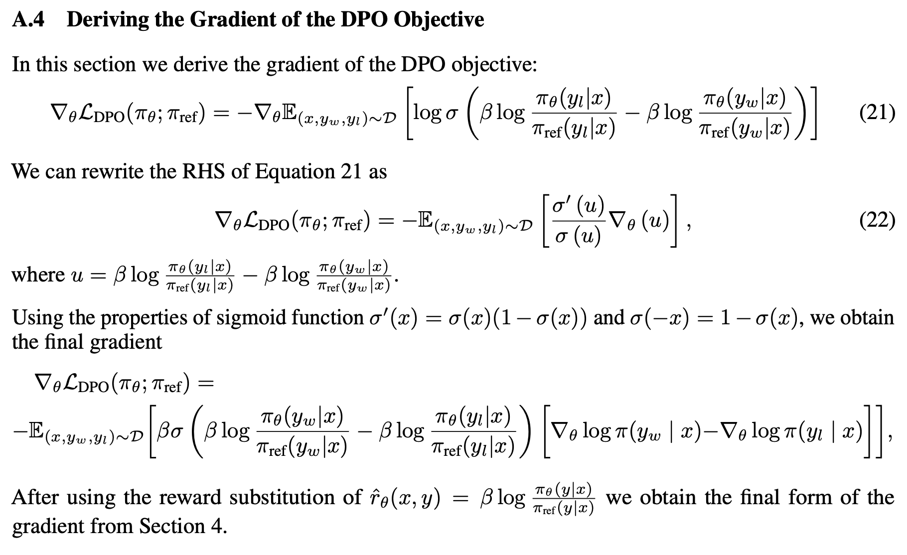
DPO paper has provided detailed steps of deriving the gradient of the DPO objective: (Source: Direct Preference Optimization: Your Language Model is Secretly a Reward Model)

dpo_gradients_derivation_paper

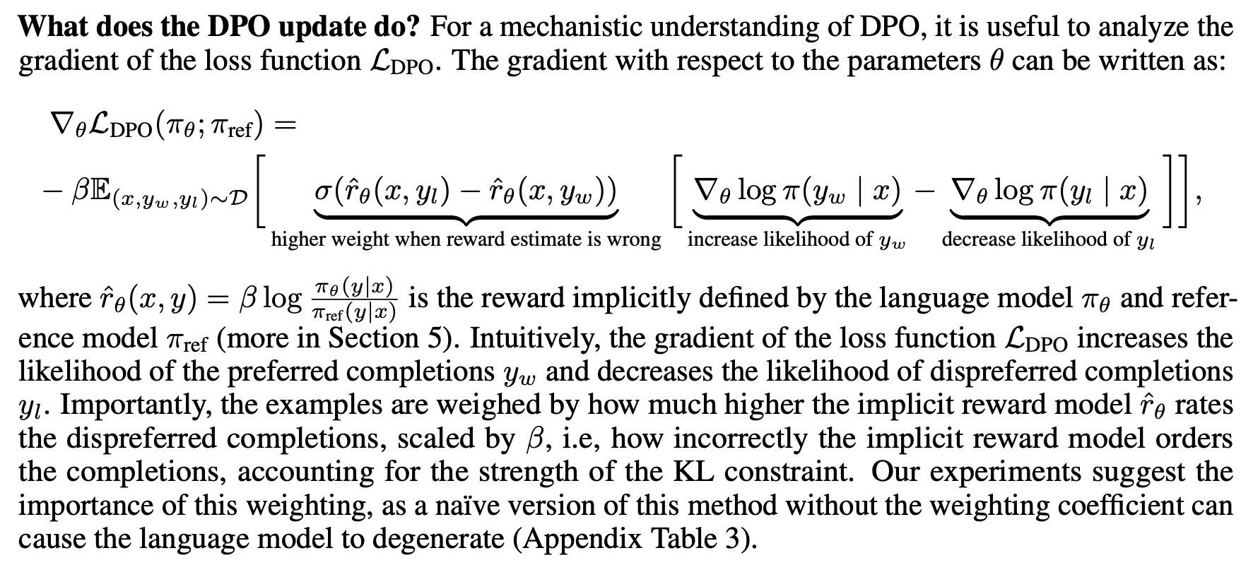
The simplified version of the DPO gradient for better understanding is written as follows. Intuitively, when the difference between \(\hat{r}_{\theta}(x, y_l)\) and \(\hat{r}_{\theta}(x, y_w)\) is large, the gradient takes a larger step during optimization. Conversely, when the difference is small, the objective is optimized with a smaller adjustment.

DPO_gradient_simple_version

DPO Usage

Here's how DPO is applied step by step:

1. Initial Setup and Supervised Fine-Tuning (SFT): Begin by fine-tuning a pre-trained LLM using supervised learning on a dataset that is representative of the tasks the model will perform. This step ensures the model has a strong foundation in the relevant domain, preparing it for preference-based optimization.

2. Collect Preference Data: Gather human feedback in the form of pairwise preferences or rankings. Annotators evaluate responses generated by the model and indicate which ones they prefer. Construct a dataset of prompts and corresponding preferred and less-preferred responses.

3. Iterative Rounds of DPO

• Sampling and Annotation: In each round, sample a set of responses from the model for given prompts. Collect new preference annotations based on these samples, allowing for dynamic updates to the preference dataset. (Public preference data works as well. Off-policy and on-policy data both work).

• Preference Optimization: Use DPO to adjust the model's outputs based on collected preference data:

• Model Update: Fine-tune the model using this loss function to increase the likelihood of generating preferred responses.

4. Evaluation and Iteration

• Performance Assessment: After each round, evaluate the model’s performance on new prompts to ensure it aligns with human preferences. Use feedback from these evaluations to inform subsequent rounds of sampling and optimization.

• Iterative Refinement: Continue this loop process over multiple rounds, iteratively refining the model's alignment with human preferences through continuous sampling and preference optimization.

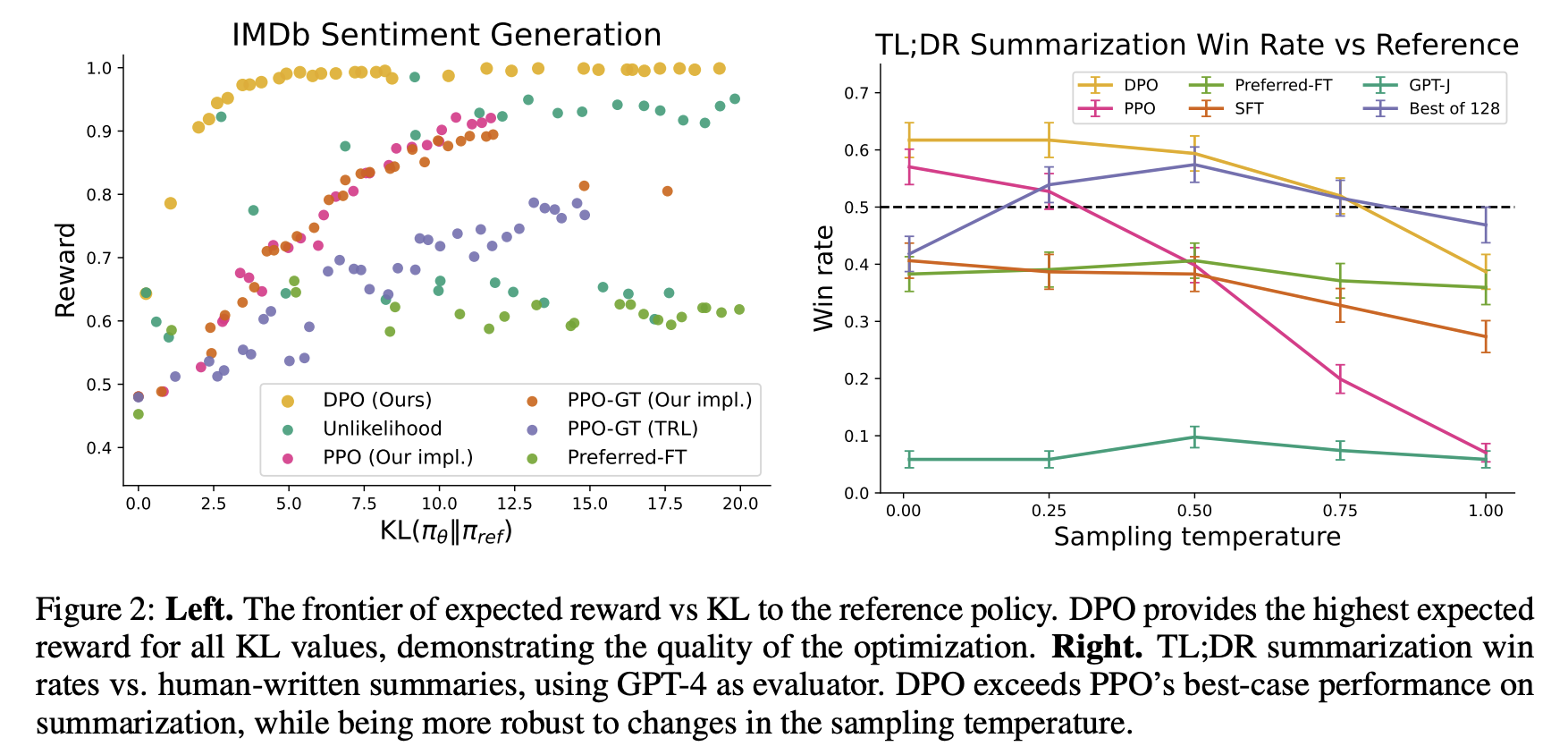
DPO Performance

(Source: Direct Preference Optimization: Your Language Model is Secretly a Reward Model)

DPO_performance_paper

DPO Objective Pseudocode

\[ L_{DPO}(\pi_\theta; \pi_{ref}) = -E_{(x,y_w,y_l) \sim D} \Big[\log \sigma \Big(\beta \log {\pi_{\theta}(y_w|x)\over \pi_{ref}(y_w|x)} - \beta \log {\pi_{\theta}(y_l|x)\over \pi_{ref}(y_l|x)}\Big)\Big)\Big] \]

import torch.nn.functional as F

def dpo_loss(pi_logps, ref_logps, yw_idxs, yl_idxs, beta):
    """
    pi_logps: policy logprobs, shape (B,)
    ref_logps: reference model logprobs, shape (B,)
    yw_idxs: preferred completion indices in [0, B-1], shape (T,)
    yl_idxs: dispreferred completion indices in [0, B-1], shape (T,)
    beta: temperature controlling strength of KL penalty

    Each pair of (yw_idxs[i], yl_idxs[i]) represents the
    indices of a single preference pair.
    """

    pi_yw_logps, pi_yl_logps = pi_logps[yw_idxs], pi_logps[yl_idxs]
    ref_yw_logps, ref_yl_logps = ref_logps[yw_idxs], ref_logps[yl_idxs]

    pi_logratios = pi_yw_logps - pi_yl_logps
    ref_logratios = ref_yw_logps - ref_yl_logps

    losses = -F.logsigmoid(beta * (pi_logratios - ref_logratios))
    rewards = beta * (pi_logps - ref_logps).detach()

    return losses, rewards

DPO Variants

The key area of research involves developing variants of DPO and conducting theoretical analyses to understand its limitations and potential improvements. This includes exploring different loss functions or optimization strategies that can be applied within the DPO framework.

• One significant area of research focuses on refining the loss function used in DPO. This includes exploring ways to eliminate the need for a reference model, which can simplify the optimization process.

  Examples:

  • ORPO: Monolithic Preference Optimization without Reference Model

  • SimPO: Simple Preference Optimization with a Reference-Free Reward

• Another key direction involves leveraging existing supervised fine-tuning data as preference data for DPO. This strategy aims to enhance the quality of preference data by utilizing high-quality labeled datasets that may already exist from previous SFT processes.

  Examples:

  • Refined Direct Preference Optimization with Synthetic Data for Behavioral Alignment of LLMs

Main Difficulties in RLHF

Data Collection

In practice, people noticed that the collection of human feedback in the form of the preference dataset is a slow manual process that needs to be repeated whenever alignment criteria change. And there is increasing difficulty in annotating preference data as models become more advanced, particularly because distinguishing between outputs becomes more nuanced and subjective.

• The paper “CDR: Customizable Density Ratios of Strong-over-weak LLMs for Preference Annotation” explains that as models become more advanced, it becomes harder to identify which output is better due to subtle differences in quality. This makes preference data annotation increasingly difficult and subjective.
• Another paper, “Improving Context-Aware Preference Modeling for Language Models,” discusses how the underspecified nature of natural language and multidimensional criteria make direct preference feedback difficult to interpret. This highlights the challenge of providing consistent annotations when outputs are highly sophisticated and nuanced.
• “Less for More: Enhancing Preference Learning in Generative Language Models” also notes that ambiguity among annotators leads to inconsistently annotated datasets, which becomes a greater issue as model outputs grow more complex.

Reward Hacking

Reward hacking is a common problem in reinforcement learning, where the agent learns to exploit the system by maximizing its reward through actions that deviate from the intended goal. In the context of RLHF, reward hacking occurs when training settles in an unintended region of the loss landscape. In this scenario, the model generates responses that achieve high reward scores, but these responses may fail to be meaningful or useful to the user.

In PPO, reward hacking occurs when the model exploits flaws or ambiguities in the reward model to achieve high rewards without genuinely aligning with human intentions. This is because PPO relies on a learned reward model to guide policy updates, and any inaccuracies or biases in this model can lead to unintended behaviors being rewarded. PPO is particularly vulnerable to reward hacking if the reward model is not robustly designed or if it fails to capture the true objectives of human feedback. The iterative nature of PPO, which involves continuous policy updates based on reward signals, can exacerbate this issue if not carefully managed.

DPO avoids explicit reward modeling by directly optimizing policy based on preference data. However, it can still encounter issues similar to reward hacking if the preference data is biased or if the optimization process leads to overfitting specific patterns in the data that do not generalize well. While DPO does not suffer from reward hacking in the traditional sense (since it lacks a separate reward model), it can still find biased solutions that exploit out-of-distribution responses or deviate from intended behavior due to distribution shifts between training and deployment contexts.

• The article "Reward Hacking in Reinforcement Learning" by Lilian Weng discusses how reward hacking occurs when a RL agent exploits flaws or ambiguities in the reward function to achieve high rewards without genuinely learning the intended task. It highlights that in RLHF for language models, reward hacking is a critical challenge, as models might learn to exploit unit tests or mimic biases to achieve high rewards, which can hinder real-world deployment.
• The research "Scaling Laws for Reward Model Overoptimization" explores how optimizing against reward models trained to predict human preferences can lead to overoptimization, hindering the actual objective.
  1. Impact of Policy Model Size: Holding the RM size constant, experiments showed that larger policy models exhibited similar overoptimization trends as smaller models, despite achieving higher initial gold scores. This implies that their higher performance on gold rewards does not lead to excessive optimization pressure on the RM.
  2. Relationship with RM Data Size: Data size had a notable effect on RM performance and overoptimization. Models trained on fewer than ~2,000 comparison labels showed near-chance performance, with limited improvement in gold scores. Beyond this threshold, all RMs, regardless of size, benefited from increased data, with larger RMs showing greater improvements in gold rewards compared to smaller ones.
  3. Scaling Laws for RM Parameters and Data Size: Overoptimization patterns scaled smoothly with both RM parameter count and data size. Larger RMs demonstrated better alignment with gold rewards and less susceptibility to overoptimization when trained on sufficient data, indicating improved robustness.
  4. Proxy vs. Gold Reward Trends: For small data sizes, proxy reward scores deviated significantly from gold reward scores, highlighting overoptimization risks. As data size increased, the gap between proxy and gold rewards narrowed, reducing overoptimization effects.

Note that the KL divergence term in the RLHF objective is intended to prevent the policy from deviating too much from a reference model, thereby maintaining stability during training. However, it does not fully prevent reward hacking. Reward hacking occurs when an agent exploits flaws or ambiguities in the reward model to achieve high rewards without genuinely aligning with human intentions. The KL divergence penalty does not correct these flaws in the reward model itself, meaning that if the reward model is misaligned, the agent can still find ways to exploit it. KL does not directly address whether the actions align with the true objectives or desired outcomes.